Lab 9: Mapping
The goal of this lab was to construct a map of the robots environment, which will crucial to localizing the robot for later labs. The main approach for this lab was to rotate the robot and read out depth measurements from the ToF sensors, similar to a LiDAR scan.
Angular Velocity Control
Before reading out distance measurements, the robot needed a reliable way of rotating in place or at least on some fixed axis in a predictable way.
Although this could be implemented using orientation control on yaw, the concern was that the drift from integrating gyroscope measurements would make these measurements very inaccurate over a long enough period of time. This would especially become more of a problem if the robot moves very slow to acquire a higher resolution of the map.
For this reason, a PID controller on the angular velocity of the robot was instead implemented, which hopefully would circumvent integrating the gyroscope readings:
float yaw_vel_setpoint = 0;
float f_gz = 0;
void yaw_vel_control(){
  float windup_cap = 100000;
  float beta = 0.25;
  f_gz = beta*gz[previdx] + (1-beta)*f_gz;
  float error = yaw_vel_setpoint-gz[previdx];

  if (abs(sum_error + error*h) <= windup_cap) {
    sum_error += error*h;
  }

  float alpha = 0.25;
  float diff_error = (error - prev_error)/h;
  prev_error = error;
  f_diff_error = alpha*diff_error + (1-alpha)*f_diff_error;

  float p_term = KP*error;
  float i_term = KI*sum_error;
  float d_term = KD*f_diff_error;
  int pwm = round(p_term + i_term + d_term);

  pwml = -pwm;
  pwmr = 0;
  writepwm(pwml,pwmr,40);
}
While implementing the controller, it was observed that rotating along the robot’s center axis was especially difficult at slow angular velocities, as one of the motors would potentially stall while the other would turn without any predictable pattern. Since these asymmetries in motor performance would easily throw the rotation off the center axis, the right motor was held still so that the robot would turn around an axis centered between the left wheels.
Furthermore, because the vibrations of the motors could add significant amounts of noise to the gyroscope while moving, a complementary low pass filter was applied to the readings. Granted, this would make the sensor readings slower to sharp transitions in angular velocity, but this is not really a concern since the goal is to move as slowly as possible.
After tuning the controller, it was found that the slowest velocity that could be achieved was about 50 degrees per second, where the corresponding PID parameters were $K_P = 3.0$, $K_I = 0.001$, and $K_D = 0.0$.
Assuming a sampling period of roughly 20 milliseconds (the measurement time budget in the “long” mode) for each distance sensor, this would correspond to 50 sensor readings per second and 360 sensor readings per rotation. If both ToF sensors are used, then this rate would essentially be doubled, although this would require finding the transformation matrices for both sensors precisely.
Although this might imply a very high mapping resolution, we note that the robot is constantly moving during each sensor measurement and hence the accuracy of each distance measurement would be somewhat lower. In a 4 meter-by-4 meter empty square room, the distance measurements roughly behave with the secant of the angle. This implies that we might find the greatest rate of change in distance around the corners, so in the worst case we would expect a distance change of about
\[\begin{align} 4\left(\sec\left(45 \text{ deg} - \frac{50 \text{ deg}/\text{s}}{50 \text{samples}/\text{s}}\right)\right) &= 0.09620 \text{ m} \end{align}\]If we assume that this distance change is simply added to the ToF distance reading, we would expect roughly a 100 mm worst case error. While this might seem like a lot, the relative error of the measurement is still below about 5%, and the accuracy is substantially improved when near the middle of the walls and not the corners. In reality however, we observe worse accuracy at longer distances, so this might have to be offset with some correcting factor in the actual data.
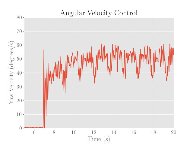
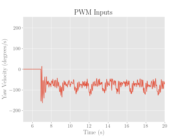
Below we demonstrate the performance of the controller:
 |
 |
Note that to reduce the friction associated from the wheels skidding, a generous amount of duct tape was applied to the wheels, which can be seen from the video above.
Furthermore, although the robot could potentially move slower, the noise of the gyroscope readings as seen in the figure above range up to 20 degrees per second from the nominal setpoint of 50 degrees per second. Since this would essentially mean a relative error of nearly 80% at 25 degrees per second, the setpoint velocity was increased to hopefully reduce the errors in the angular velocity.
Finally, the gyroscope readings also demonstrate periodic dips in angular velocity, which seem to be due to the wheels getting stuck at a certain point of the rotation. This might have been because the tape was applied somewhat unevenly, or possibly due to the mechanism of the wheels or motor.
While increasing the integral term would in theory provide an extra kick in motor power to reduce the magnitude of the dips, this would also increase the overshoot on the way out of the dip, which would require a delicate balance with the dampening of the derivative term.
Unfortunately, these dips from the output never faded even after a substantial amount of tuning.
Distance Scan
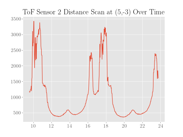
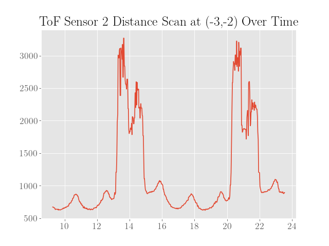
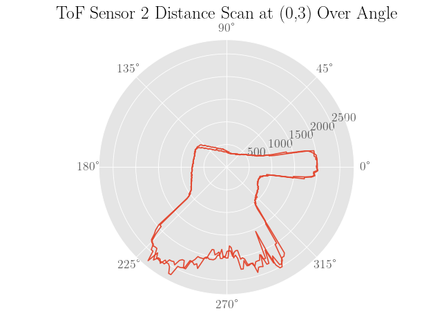
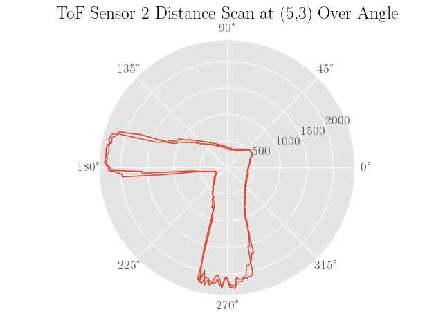
Once the controller for rotating the robot was sufficiently tuned, the robot was then placed inside a walled environment inside the lab space at the 4 coordinate points $(0,3)$, $(5,3)$, $(5,-3)$, and $(-3,-2)$, where the $x$ and $y$ axes are in meters. At each marked location, the robot was then oriented facing in the positive $y$-direction and set to rotate for at least two full turns to gauge the precision of the distance scans.
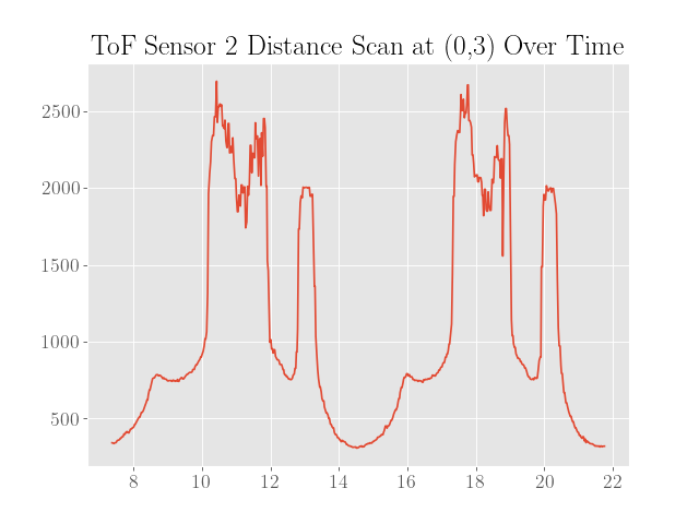
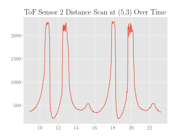
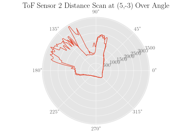
To sanity check the distance scans, plots of the distance data in polar coordinates were made where the robot was assumed to be turning in place to simplify processing the data:
 |
 |
|---|---|
 |
 |
 |
 |
|---|---|
 |
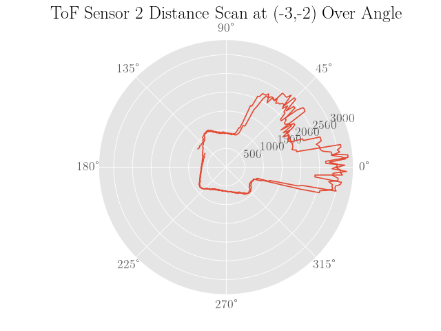 |
Also note that the angles are calculated assuming a constant angular velocity at the setpoint of 50 degrees per second and constant sampling times. Since neither of these assumptions are completely true, the plots are not expected to be very representative of the actual map.
Transformed Data
To form the map, we first need the translation matrix to convert the sensor measurements into the coordinate with respect to the center of the robot. Note that we assume that the $x$-axis of the robot is aligned with the front of the robot.
Since the ToF sensor is roughly 70 mm in front of the center and 10 mm to the right of the center, we know that the corresponding transformation in homogeneous coordinates is
\[\begin{align} T_{S}^{B} &= \begin{bmatrix} 1 & 0 & 70 \\ 0 & 1 & 10 \\ 0 & 0 & 1 \end{bmatrix} \end{align}\]Finally, we perform one more coordinate transformation to translate to the center of rotation, which is roughly 70 mm to the right of the robot’s center:
\[\begin{align} T_{B}^{C} &= \begin{bmatrix} 0 & 0 & 0 \\ 0 & 0 & 70 \\ 0 & 0 & 1 \end{bmatrix} \end{align}\]Next, we construct the rotation matrix to align the axes of the body fixed frame to the global frame, which is a function of the robot’s angular pose $\theta$ relative to the global coordinate axes:
\[\begin{align} R_{B}^{G}(\theta) &= \begin{bmatrix} \cos(\theta) & -\sin(\theta) \\ \sin(\theta) & \cos(\theta) \end{bmatrix} \end{align}\]We can then find the coordinates of the ToF measurement in the global reference frame via
\[\begin{align} \tilde{P}^{C} &= T_{B}^{C}T_{S}^{B}\tilde{P}^{S} \\ P^{G} &= R_{B}^{G}P^{C} \end{align}\]Here, we define $P^{S}$ to be the distance measurement, which is in the sensors reference frame:
\[\begin{align} P^{S} &= \begin{bmatrix} d \\ 0 \end{bmatrix} \\ \tilde{P}^{S} &= \begin{bmatrix} P^{S} \\ 1 \end{bmatrix} \\ \tilde{P}^{C} &= \begin{bmatrix} P^{C} \\ 1 \end{bmatrix} \end{align}\]Note that $d$ is the reading from the ToF sensor, which is aligned with the sensor reference frame’s $x$-axis.
We then implement this in Python as the following:
T_SB = np.array([[1, 0, 70],[0, 1, 10],[0, 0, 1]])
T_BC = np.array([[1, 0, 0],[0, 1, 70],[0, 0, 1]])
def R_BG(theta):
    return np.array([[np.cos(theta), np.sin(theta)],[-np.sin(theta), np.cos(theta)]])
def P_G(d,theta):
    P_Sh = np.array([[d],[0],[1]])
    P_Ch = T_BC.dot(T_SB.dot(P_Sh))
    P_C = P_Ch[0:-1]
    P_G = R_BG(theta).dot(P_C)
    return P_G
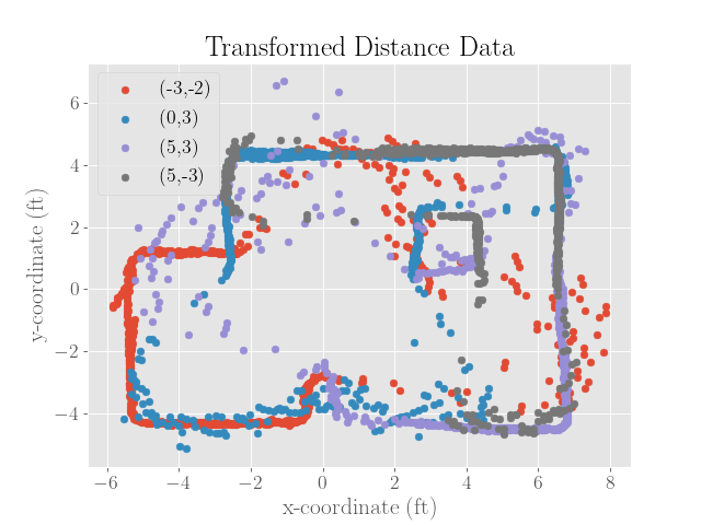
After merging the scans together, we get the following map, which is plotted in both feet and millimeters:
 |
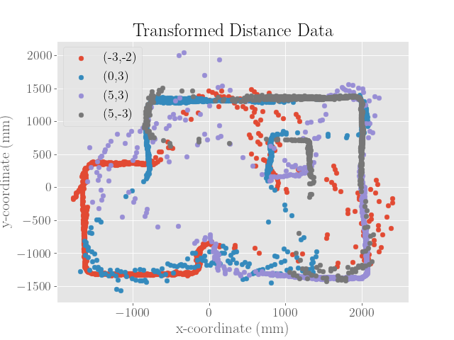 |
To get the merged map, I had to adjust the initial angle until the map segment seemed to rotate nicely into place. Although I made sure to orient the robot at the same angle at each of the marked locations, I didn’t mark the timestamp at the moment the PID controller was engaged. To find the starting of the PID control, I simply adjusted the indexes of the received data until the data seemed periodic with two periods.
However, the lack of synchronization doesn’t fully explain the changing initial angle if two full periods were recorded. A second reason would then be the rise time of the angular velocity upon starting up the PID controller, which might result in the robot moving slowly or not at all for a brief period of time.
Mapping
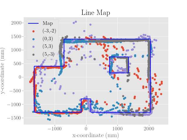
To form the line-based map, I tried to make straight lines out of the plotted ToF distance data. In general, I trusted measurements that were closer to the robot’s center of rotation.
 |
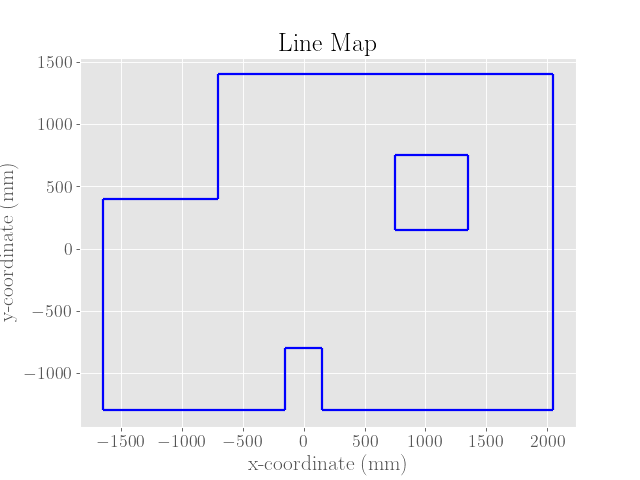 |
For reference, the list of line segments used to form the map are included below:
# Walls
[(-1650, -1300), (-150, -1300)],
[(-1650, -1300), (-1650, 400)],
[(-1650, 400), (-700, 400)],
[(-700, 400), (-700, 1400)],
[(-700, 1400), (2050, 1400)],
[(2050, 1400), (2050, -1300)],
[(2050, -1300), (150, -1300)],

# Box 1
[(150, -1300), (150, -800)],
[(150, -800), (-150, -800)],
[(-150, -800), (-150, -1300)],

# Box 2
[(750, 750), (750, 150)],
[(750, 750), (1350,750)],
[(1350, 750), (1350, 150)],
[(750, 150), (1350, 150)]