Lab 8: Stunts
The goal of this lab was to essentially put together the PID controller and Kalman filter to execute high speed stunts with the robot.
In this instance, the objective was to drive quickly towards a wall about 3 m away, perform a flip, and then drive back as fast as possible back to the starting line.
Kalman Filter Speedup
To pull of the stunt, it was critical to get somewhat accurate readings of the distance to the wall as fast as possible. Considering that the measurement budget of the ToF sensor in the long range mode is over 30 ms, and considering that the robot reaches top speeds of around 2000 mm/s, a late measurement upon reaching the setpoing of 500 mm from the wall would potentially result in up to (2000)(0.03) = 60 mm of additional error.
Combined with additional errors from sensor noise or bias (\(\pm\)20 mm according to the datasheet), this could potentially result in up to 80 mm of error in the worst case. Admittedly, this analysis is still a little too optimistic, as several failed runs have resulted in the robot crashing in the wall due to control loop latency.
To address this issue, the Kalman filter was used to predict measurements for several iterations between each sensor measurement. This was accomplished by splitting the Kalman filter into two functions, which was done in the previous lab. For reference, we include a code snippet below:
void kf_pred_step(float u){
  Matrix<1,1> u_matrix = {u};
  mu = A_d * mu + B_d * u_matrix;
  Sigma = A_d * Sigma * ~A_d + Sigma_u;
}

void kf_update_step(float z){
  Matrix<1,1> Sigma_m = C * Sigma * ~C + Sigma_z;
  Invert(Sigma_m);
  Matrix<2,1> K_kf = Sigma * ~C * Sigma_m;
  Matrix<1,1> z_matrix = {z};
  Matrix<1,1> z_m = z_matrix - C*mu;
  mu = mu + K_kf*z_m;
  Sigma = (I - K_kf*C) * Sigma;
}
The naive approach to achieving the speedup would be to essentially run the prediction step until the distance measurements were ready according to the checkForDataReady() function, where the update step would then be called.
However, the issue with this approach is that the latency of the calls to simply verify whether the measurements were ready would easily take up to 20 ms of latency, so no actual speedup would be achieved.
The workaround to this was to essentially omit any calls to checkForDataReady(), and to simply read measurements every 8 iterations. However, because this poses the risk of not giving the ToF sensor enough time to complete the measurement, a minimum duration of each loop iteration of 4 ms was enforced, which provided a measurement time budget of around 32 ms:
while (central.connected()) {
        // Sampling Rate
        if (millis() - initial >= 4) {
          // Handle command
          handle_command();

          // KF Prediction
          kf_pred_step(pwml/100.0);

          if (skipidx == 0) {
            d2[idx] = distanceSensor2.getDistance();

	    // KF Update
            kf_update_step(d2[idx]);
          }
          else {
            d2[idx] = -1;
          }

          // Time
          initial = millis();
          t[idx] = initial;


          // KF
          kf_pos[idx] = mu(0,0);
          kf_vel[idx] = mu(1,0);

          // Motor
          ml[idx] = pwml;
          mr[idx] = pwmr;

          // PID
          KP_val[idx] = KP;
          KI_val[idx] = KI;
          KD_val[idx] = KD;

          previdx = idx;
          idx = (idx + 1)%MAX_SIZE;
          skipidx = (skipidx + 1)%skipcount;
      }
    }
Using this approach, an average loop latency of around 8-10 ms was easily achieved, which was around half the previous latency of 16 ms before the speedup.
However, the relative variability of the latency also increased, which was easily around 4-5 ms. Since this would essentially mean a 50 % error in the timesteps $h$ in the PID controller and Kalman filter when approximating derivatives and integrals, the assumption of a constant sampling rate didn’t seem to hold that well.
To address this, a variable timestep $h$ was updated every iteration and incorporated into the PID controller and Kalman filter. This admittedly did require a bit of retuning of the PID constants, but was fairly easy since the ballpark estimates were already known previously for constant time steps.
// Timestep
h = (t[idx] == t[previdx]) ? 4 : (t[idx]-t[previdx]);

H = {h/1000, 0,
     0, h/1000};
A_d = I + H*A;
B_d = H*B;
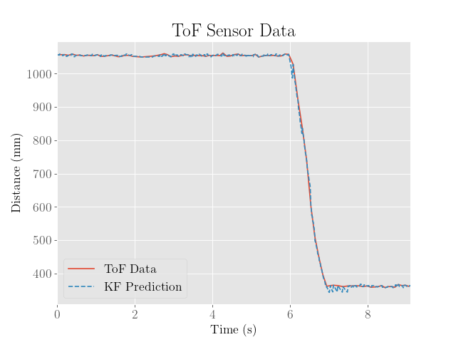
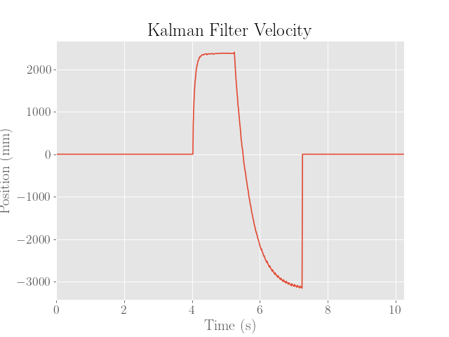
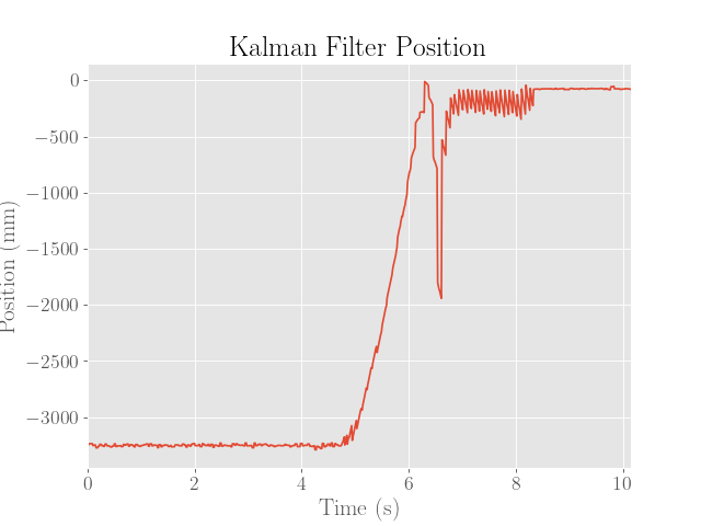
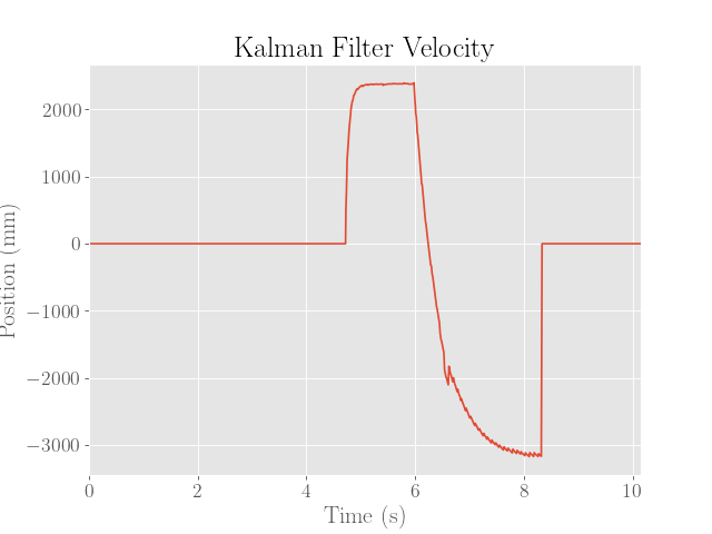
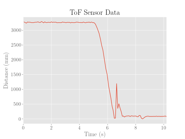
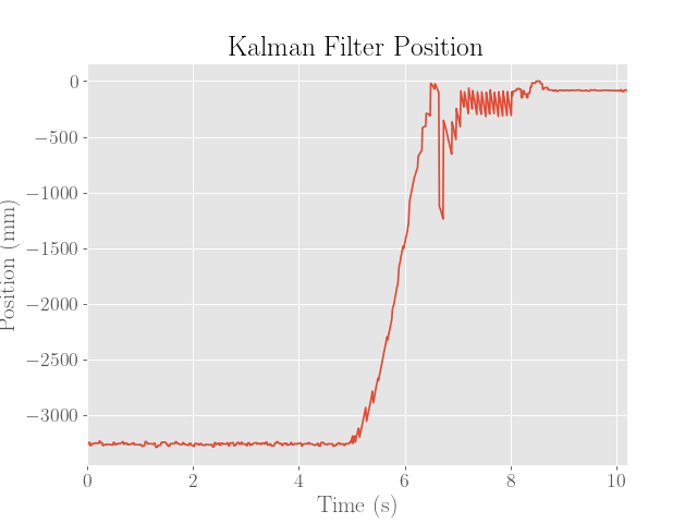
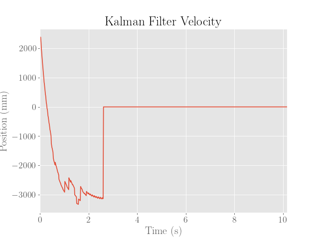
For reference, the estimates produced by the Kalman filter with the PID controller are provided below:
Velocity PID Control
Once the Kalman filter was producing reasonable estimates of the distance to the wall even with the sped up loop, the next step was to implement a simple PID controller for the velocity of the robot tto make the robot head towards the wall at a robust, predictable speed.
While a faster solution might be to simply apply the maximum power to the motors, this might result in the robot crashing into the wall if the loop speed is still too slow, so setting a predictable speed would be more helpful for testing the stunt. The implementation of the PID controller was essentially the same as the position controller, albeit with a difference setpoint and sign for the error.
Note that the second entry of the Kalman filter’s state (representing velocity) is used.
void vel_control(){
  float setpoint = 2500;
  float windup_cap = 10000;
  float error = setpoint-mu(1,0);

 if (abs(sum_error + error*h) <= windup_cap) {
    sum_error += error*h;
  }

  float alpha = 0.25;
  float diff_error = (error - prev_error)/h;
  prev_error = error;
  f_diff_error = alpha*diff_error + (1-alpha)*f_diff_error;

  float p_term = KP*error;
  float i_term = KI*sum_error;
  float d_term = KD*f_diff_error;
  int pwm = round(p_term + i_term + d_term);

  pwml = pwm;
  pwmr = pwm;
  writepwm(pwml,pwmr);
}
After a bit of tweaking PID constants of KP = 0.6, KI = 0.001, and KD = 5 seemed to produce minimal overshoot and oscillations.
Stunt
The final step of the stunt was to perform the flip. The naive approach was to simply apply active braking by setting both motor PWM inputs to high. Unfortunately, this did not seem to work that well, and would also be slower since the robot would need to drive back as well.
The fix was to simply send commands to drive the motor backwards, in the hopes that the rapid change in momentum would cause the flip:
if (-mu(0,0) <= 1000 || flipped) {
  // Flip
 pwml = -custom_pwm+epsilon;
 pwmr = -custom_pwm-epsilon;
 writepwm(pwml,pwmr,40);
 flipped = true;
 break;
}
vel_control();
The solution was to shift the weight distribution of the robot so that the center of mass was sufficiently shifted off the center, which made the flip much easier. This was easily accomplished by moving the batteries to the front of the robot, which required a bit of resoldering of the connectors to fit everything in the front compartment.
Once this was achieved however, the flip became pretty easy to pull off. The only remaining concern was how reliably the robot could drive backwards in a straight path back to the starting line, as any slight bias between the left and right motors would easily result in the robot veering off to the side after the flip.
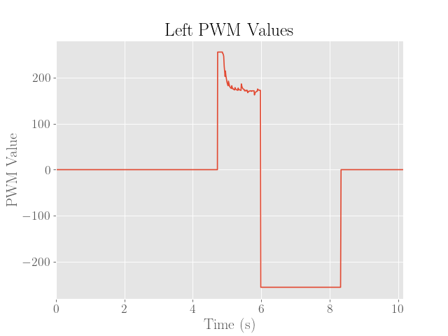
While a robust fix would be to somehow perform PID control on the orientation of the robot, the fix in this case was just to add a small correcting factor (epsilon) to the pwm values, which would hopefully minimize the chances of an angled return path. After a bit of tweaking, the optimal values seemed to be a left motor PWM value of -255 and a right motor PWM value of -235.
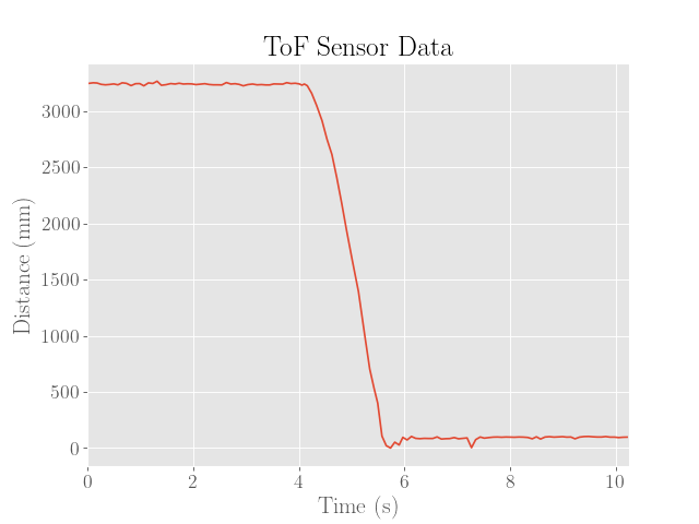
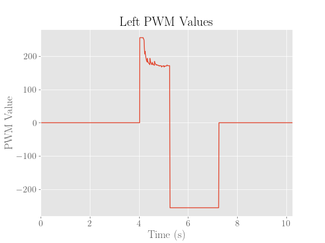
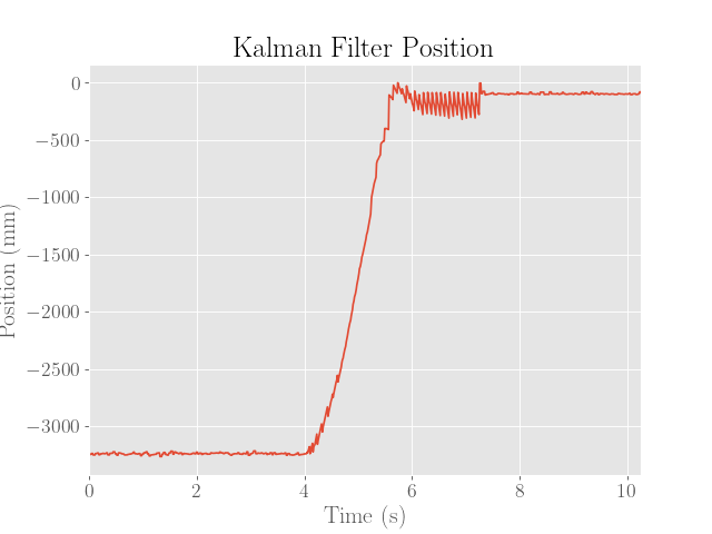
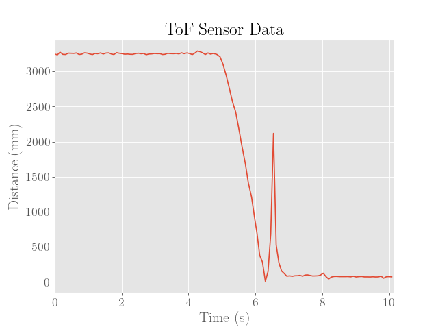
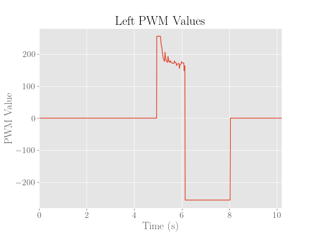
The final executions of the stunt are then shown below. Note that for brevity, only the left motor PWM values are shown since the values are virtually the same except for a small correcting factor.
 |
 |
|---|---|
 |
 |
 |
 |
|---|---|
 |
 |
 |
 |
|---|---|
 |
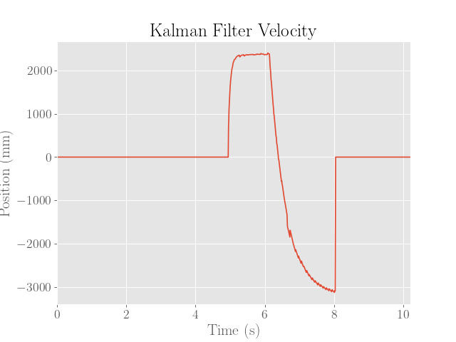 |
I’m pretty sure this last one doesn’t really count as a successful run”, but I guess it counts as a blooper?
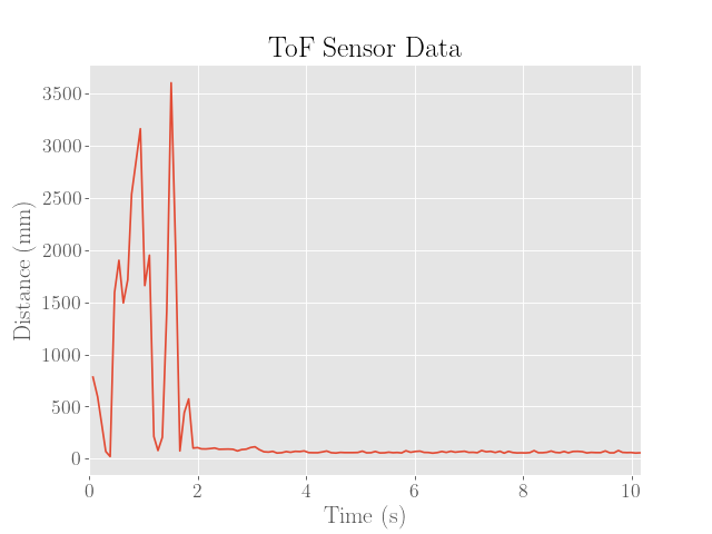 |
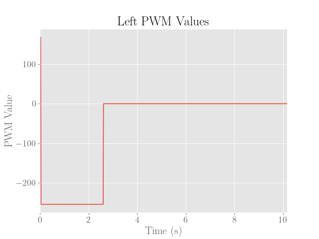 |
|---|---|
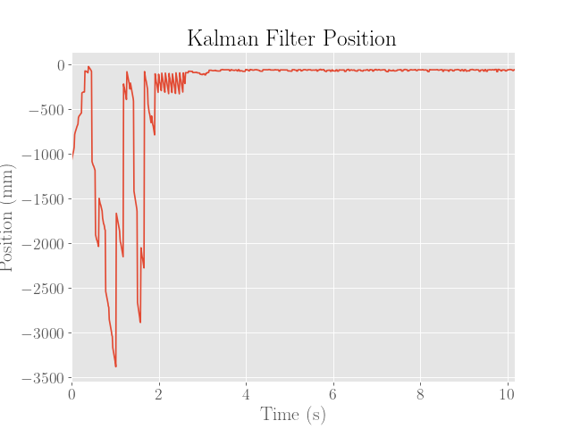 |
 |
As a fair disclaimer, the methods used to execute this stunt are incredibly far from being robust (the true success rate is probably no greater than 1 out of every 5 attempts). While the flip happens rather consistently, the real issue was in the inability of the robot to regulate its orientation.
As shown in the video, the speed of the robot tends to make it bounce after the flip, which tends to make the robot veer off to the side. Another issue that wasn’t fully resolved was how the flip could land at an angle, which caused the robot to completely miss the finish line on the way back.
Since slippage of the wheels, bouncing, and disturbances to the robot are all generally things that occur at high speeds, the only real solution under this “semi-open-loop” control approach would be to lower the speed. To truly produce a robust solution however, some degree of orientation control would have to be implemented, so that the robot could either flip, reorient, and then return, or to possibly dynamically steer while moving back for an even faster solution.
The last solution requires creating a controller for a nonlinear system, so techniques such as feedback linearization might prove to be more useful in this case.
Speed
Finally, to estimate the total time elapsed from the start to finish of the stunt, the duration of when the robot first crosses the starting line and last crosses the line was estimated from the video:
| Attempt | Time Elapsed (s) |
|---|---|
| 1 | 2.90 |
| 2 | 3.02 |
| 3 | 3.03 |
| Average | 2.98 |