Lab 7: Kalman Filter
This lab was dedicated to implementing a Kalman filter, which will help extrapolate the collected sensor measurements and help reduce the latency between each input to the PID controller.
System ID
Before implmenting the Kalman filter, it was crucial to first identify the state equations associated with the position $x$ of the robot. These are chararacterized by a simple drag equation with input velocities $u$, which is stated as follows:
\[\begin{align} \begin{bmatrix} \dot{x} \\ m\ddot{x} \end{bmatrix} &= \begin{bmatrix} x \\ -d\dot{x} + u \end{bmatrix} \end{align}\]This can then be expressed as the following linear state space equation:
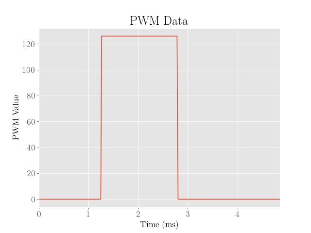
\[\begin{align} \begin{bmatrix} \dot{x} \\ \ddot{x} \end{bmatrix} &= \begin{bmatrix} 0 & 1 \\ 0 & -\frac{d}{m} \end{bmatrix} \begin{bmatrix} x \\ \dot{x} \end{bmatrix} + u \begin{bmatrix} 0 \\ \frac{1}{m} \end{bmatrix} \end{align}\]Here, the drag $d$ and mass $m$ of the robot are not initially known, and must be measured via taking the step response of the system. This was done by sending a stream of constant PWM values to the motors.
This was basically accomplished by setting the PWM values of the robot to the maximum values achieved using the position PID controller developed in Lab 6, which were around 100 before shifting and rescaling to account for the motor’s PWM deadband.
These values were taken before the deadband (output of the PID controller) so that the input behave linearly (the shifting out of the deadband is affine). Admittedly, this probably doesn’t make a huge difference anyway.
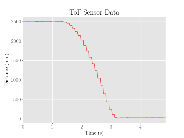
The ToF sensor data was then collected as the robot approached a wall, and the resulting sensor outputs, motor inputs were plotted.
 |
 |
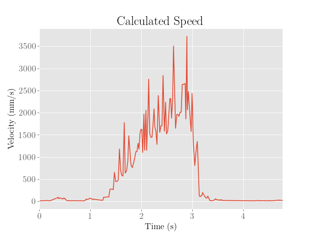
The speed of the robot was also estimated by taking finite differences of the ToF data. However, the ToF sensor data shows up as constant values over significant intervals of time, suggesting that the depth values are failing to update fast enough.
To ensure that the calculated finite differences do not vary too much, a moving average with a window size of 5 samples was taken on the ToF data in order to smooth the data out. Despite this, the calculated finite differences still demonstrated wild fluctuations, making it difficult to interpret the steady-state value.
To fix this, a second moving average filter with a window size of 10 samples was taken on the finite differences, and the peak value was interpreted as the steady-state speed, which was approximately 2271 mm/s.
This approach admittedly was a bit hacky and is most likely an underestimate of the actual steady state speeds, as the robot did not have enough time to appreciably plateau in speed. Furthermore, the introduction of moving average filters may have also smoothed out fast transitions in the depth data that may have been due to the actual movement of the robot, rather than noise in the sensor.
 |
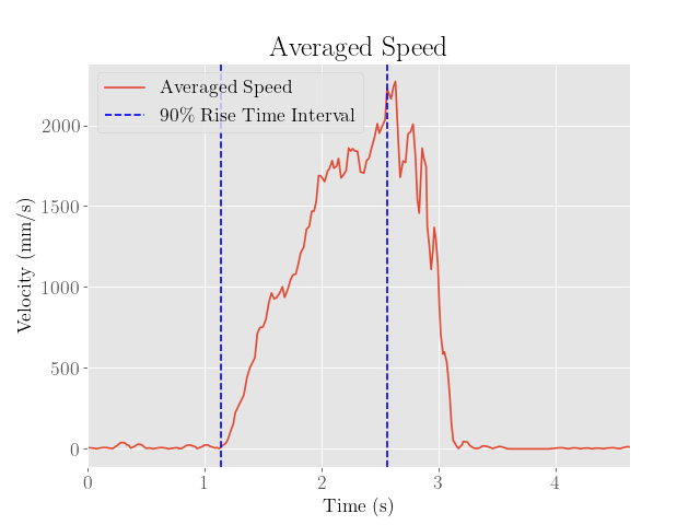 |
We then find the 90% rise time, which comes out to around 1.420 seconds, where the time interval chosen is indicated on the averaged speed graph.
From here we note that in the steady state, the acceleration is zero. Hence,
\[\begin{align} 0 &= -\frac{d}{m}\dot{x} + \frac{u}{m} \\ d &= \frac{u}{\dot{x}} \end{align}\]Using a normalized control input velocity $u = 1$ (corresponding to a PWM value of 126), we then find that the drag coefficient is approximately $d = 0.0004403$.
To find the mass value, we note that
\[\begin{align} \ddot{x} &= -\frac{d}{m}\dot{x} + \frac{u}{m} \\ \dot{x} &= \frac{u}{d} - C\exp\left(-\frac{d}{m}t\right) \end{align}\]Since the robot is initially motionless, we know that $C = \frac{u}{d}$ to ensure that $\dot{x}(t) = 0$, which is the steady state velocity. After normalizing the velocity to $v$ by dividing out the steady state velocity, this becomes
\[\begin{align} v &= 1 - \exp\left(-\frac{d}{m}t\right) \\ -\frac{d}{m}t &= \ln(1-\dot{x}) \\ m &= -\frac{dt_{0.9}}{\ln(1-0.9)} \end{align}\]Using the values of the 90% rise time and the drag coefficient calculatd earlier, we find that $m = 0.0002716$.
Since the drag coefficient could depend quite heavily on the kind of surface the robot is traveling on, the process was repeated on a smoother floor:
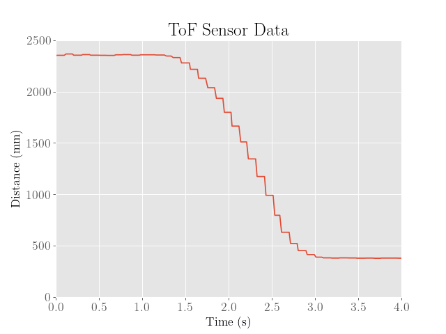 |
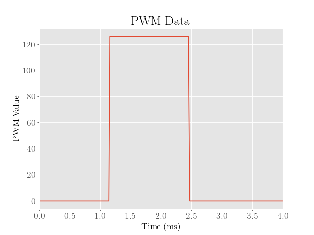 |
We then calculate the steady-state speed using the same approach as before, which comes out to around 2049 mm/s:
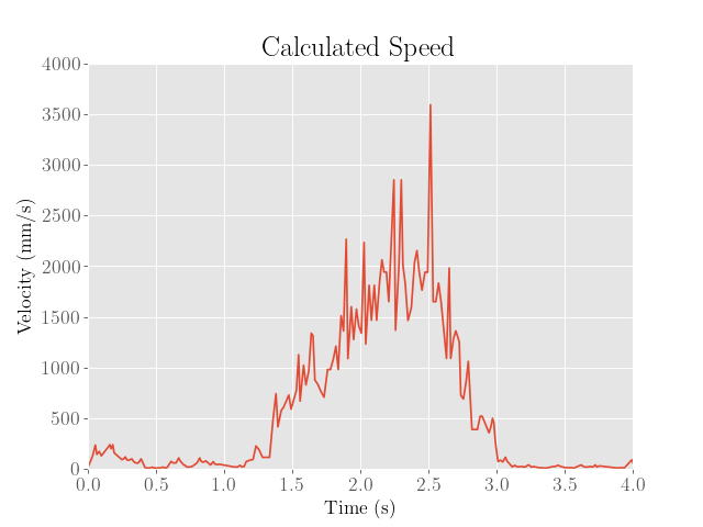 |
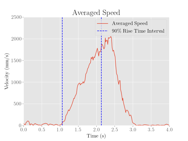 |
We also obtain a 90% rise time of around 1.078 seconds. This corresponds to a drag coefficient of $d = 0.0004880$ and a mass value of $m = 0.0002285$. Although the friction is significantly reduced in this setting, the parameters do not seem to change very drastically.
Setup
After characterizing the necessary system parameters, we then obtain the following matrices to describe the state space equation:
\[\begin{align} x_{t+1} &= Ax_t + Bu_t \end{align}\]Here, the state is defined as
\[\begin{align} x_t &= \begin{bmatrix} p_t \\ v_t \end{bmatrix} \end{align}\]where $p_t$ is the position of the robot and $v_t$ is the velocity.
Using the differential equation characterized in the previous section and the finite difference relations
\[\begin{align} p_{t+1} &= p_{t} + hv_{t} \\ v_{t+1} &= v_{t} + ha_{t} \end{align}\]We have
\[\begin{align} x_{t+1} &= A_dx_{t} + B_du_{t} \end{align}\]where
\[\begin{align} A_d &= I + Ah \\ A_d &= \begin{bmatrix} 1 & h \\ 0 & 1-2.136h \end{bmatrix} \\ B_d &= Bh \\ B_d &= \begin{bmatrix} 0 \\ 3682h \end{bmatrix} \end{align}\]In addition to the system dynamics, we specify an addition measurement matrix $C$ to define the relationship between the ToF data and the depth measurements:
\[\begin{align} C &= \begin{bmatrix} -1 & 0 \end{bmatrix} \end{align}\]To ensure that the relationship is purely linear, we define the origin of the position as the wall, which would make the position equal to the negative distance measurements to the wall (since the positive direction is taken as towards the wall).
Finally, the sensor noise and system disturbance covariance matrices need to be specified, which need to be tuned to enable the filter to perform accurately.
A reasonable estimate would be to assume a standard deviation of 27.7 millimeters, which was taken from lecture. Intuitively, this makes sense since the dynamics are generally expected to be less reliable compared to the measurements.
This yields the following process noise covariance matrix:
\[\begin{align} \Sigma_u &= \begin{bmatrix} (10^2)(0.020) & 0 \\ 0 & (10^2)(0.020) \end{bmatrix} \\ \Sigma_u &= \begin{bmatrix} 2 & 0 \\ 0 & 2 \end{bmatrix} \end{align}\]Furthermore, we also assume a standard deviation of 20 mm for the sensor noise ($\Sigma_z = 20^2$), which agrees with the ToF sensor datasheet.
Testing
We then attempt to implement the Kalman filter, which is given by the following set of recursive equations that characterize the prediction step, where an intermediate state is predicted based off of knowledge of the system dynamics, control input, and process noise::
\[\begin{align} \overline{\mu}_{t} &= A\mu_{t-1} + Bu_t \\ \overline{\Sigma}_{t} &= A\Sigma_{t-1}A^T + \Sigma_u \end{align}\]The filter also includes an additional set of equations that characterize the update step:
\[\begin{align} K_{KF} &= \overline{\Sigma}_{t}C^T(C\overline{\Sigma}_{t}C^T+\Sigma_z)^{-1} \\ \mu_{t} &= \overline{\mu}_{t} + K_{KF}(z_{t}-C\overline{\mu}_t) \\ \Sigma_{t} &= (I - K_{KF}C)\overline{\Sigma}_{t} \end{align}\]Before implementing the Kalman filter on the Artemis board, we first test the filter in Python:
# Parameters
n = 2
h = 0.02
d = 0.0004403
m = 0.0002716
sigma_1 = 27.7
sigma_2 = 20
sigma_3 = 20

# State
x = np.array([[-tof[0]],[0]])
sigma = np.array([[sigma_3**2, 0],[0, sigma_3**2]])
outputs = np.zeros([2,len(tof)])
outputs[:,0] = x.flatten()

# Matrices
A = np.array([[0, 1],[0, -d/m]])
B = np.array([[0],[1/m]])
C = np.array([[-1,0]])
sigma_u = np.array([[sigma_1**2, 0],[0, sigma_2**2]])
sigma_z = sigma_3**2
Ad = np.eye(n) + h * A
Bd = h * B

# Kalman Filter
for i in range(1,len(tof)):
    x,sigma = kf(x, sigma, pwm[i], tof[i])
    outputs[:,i] = x.flatten()
Note that as with the implementation of the PID controller, there is the option of using the time stamps to precisely calculate the time steps $h$.
To keep things simple however, these time steps are interpreted as constant, although this will admittedly add error since the time steps have a standard deviation of a few milliseconds.
Fortunately, the performance of the filter and controller both appear surprisingly robust against variations in these time steps, so there isn’t a huge loss in accuracy.
To accomplish this, we call on a provided helper function kf(), which computes the updates of the mean and covariance of the current belief after one iteration of the filter:
def kf(mu,sigma,u,y):
    mu_p = Ad.dot(mu) + Bd.dot(u)
    sigma_p = Ad.dot(sigma.dot(Ad.transpose())) + sigma_u

    sigma_m = C.dot(sigma_p.dot(C.transpose())) + sigma_z
    kkf_gain = sigma_p.dot(C.transpose().dot(np.linalg.inv(sigma_m)))

    y_m = y-C.dot(mu_p)
    mu = mu_p + kkf_gain.dot(y_m)
    sigma=(np.eye(n)-kkf_gain.dot(C)).dot(sigma_p)

    return mu,sigma
This was then tested on data from a previous iteration of the PID controller with overshoot:
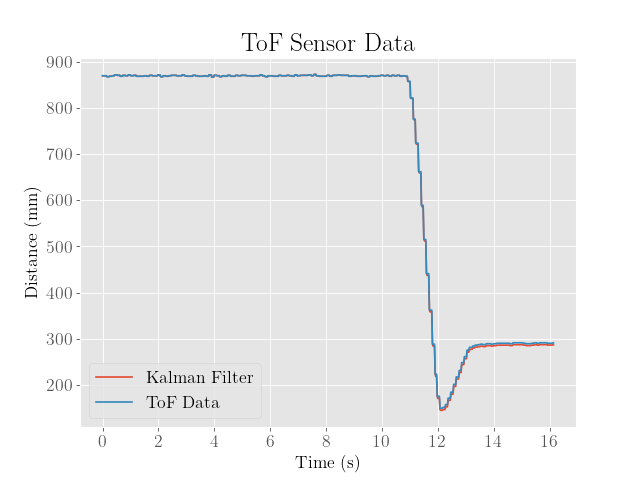 |
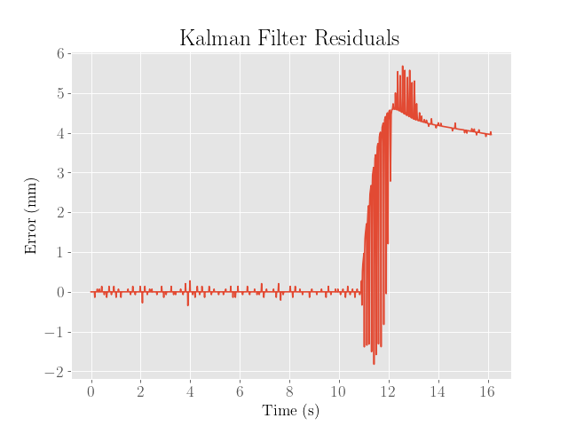 |
After both iterations, we find that the filter is nearly indistinguishable from the actual measurements, suggesting that the noise covariance values are already close to optimal, with the exception of the final predicted values, which seem to be offset by a constant error. Because the residuals are clearly biased, it seems that the system parameters were incorrectly estimated.
A solution to this was to adjust the drag coefficient to $d = 0.4403$, which was admittedly somewhat hacky, but this seemed to correct the bias. We also adjust the sensor covariance to $\Sigma_z = 1$, which significantly reduced the overall magnitude of the residuals everywhere:
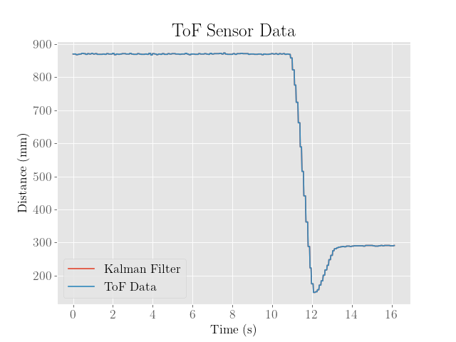 |
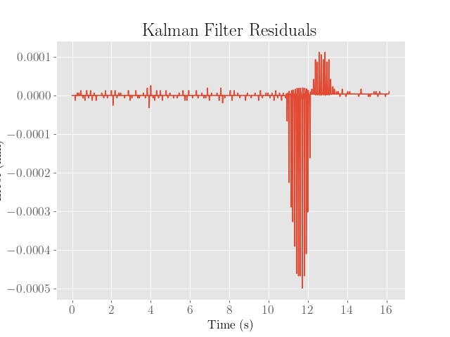 |
Note that we plot the mean of the filter and ignore the resulting covariance in this plot. We also only plot the inverted position estimate, which should equal the distance from the wall by virtue of how the origin was defined.
One danger to adjusted the system parameter $d$ is a potential overfitting of the filter and system to a particular dataset. To verify that this effect is not too egregious, we test the filter once more on the optimized PID controller data developed in Lab 6:
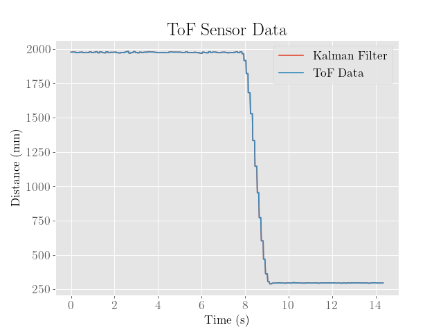 |
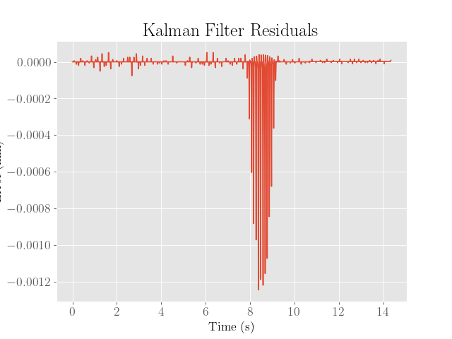 |
Note that despite the attempts to minimize the residuals, there are occassionally large spikes in error that do not seem to be explained by random noise alone, suggesting that the system parameters might still need some adjusting.
Implementation
Once the Kalman filter was verified to work in Python, the next step was to implement the filter on the robot:
Matrix<2,2> I = {1, 0,
                 0, 1};
Matrix<2,2> H = {h, 0,
                 0, h};
Matrix<2,2> A = {0, 1,
                 0, -d/m};
Matrix<2,2> A_d = I + H*A;
Matrix<2,1> B = {0,
                 1/m};
Matrix<2,1> B_d = H*B;
Matrix<1,2> C = {-1, 0};

Matrix<2,2> Sigma_u = {767.29, 0,
                      0, 767.29};
Matrix<1,1> Sigma_z = {1};

Matrix<2,1> mu;
Matrix<2,2> Sigma = I;

void kf_step(float u, float z){
  // Prediction Step
  Matrix<1,1> u_matrix = {u};
  Matrix<2,1> mu_p = A_d * mu + B_d * u_matrix;
  Matrix<2,2> Sigma_p = A_d * Sigma * ~A_d + Sigma_u;
  // Update Step
  Matrix<1,1> Sigma_m = C * Sigma_p * ~C + Sigma_z;
  Invert(Sigma_m);
  Matrix<2,1> K_kf = Sigma_p * ~C * Sigma_m;
  Matrix<1,1> z_matrix = {z};
  Matrix<1,1> z_m = z_matrix - C*mu_p;
  mu = mu_p + K_kf*z_m;
  Sigma = (I - K_kf*C) * Sigma_p;
}
To use the filter, the distance measurements were simply replaced with the filter estimates, but the key was to flip the sign since the filtered state is the negative of the measurements:
kf_step(pwml/100.0,distance2);
float error = -mu(0,0)-setpoint;
This then produced the following result:
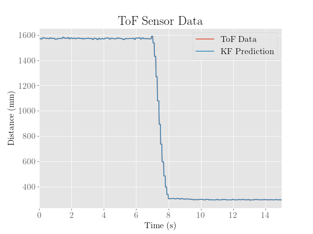 |
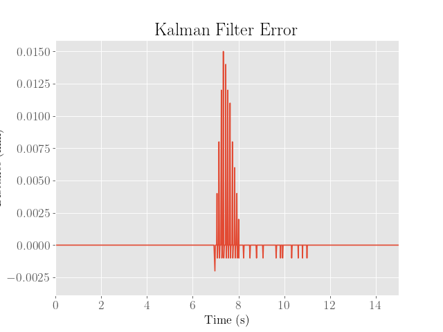 |
Speedup
Next, to use the filter to speed up the execution speed of the control loop, the key was to use the predictions of state from the filter after the prediction step alone whenever the measurements are not ready.
The idea is to essentially extrapolate to future states via the system dynamics, but in a way that incorporates the noise level and future measurements.
To do so, the filter was split into two functions:
void kf_pred_step(float u){
  Matrix<1,1> u_matrix = {u};
  mu = A_d * mu + B_d * u_matrix;
  Sigma = A_d * Sigma * ~A_d + Sigma_u;
}

void kf_update_step(float z){
  Matrix<1,1> Sigma_m = C * Sigma * ~C + Sigma_z;
  Invert(Sigma_m);
  Matrix<2,1> K_kf = Sigma * ~C * Sigma_m;
  Matrix<1,1> z_matrix = {z};
  Matrix<1,1> z_m = z_matrix - C*mu;
  mu = mu + K_kf*z_m;
  Sigma = (I - K_kf*C) * Sigma;
}
Furthermore, because the main bottleneck to the control loop’s speed is the latency due to checking for whether the sensor data is ready, these function calls are instead omitted.
However, doing so runs the risk of the sensor measurement not being ready in time, so the loop was intentionally programmed to only take a measurement periodically after a set number of iterations.
In doing so, additional errors would be added from extrapolating the dynamics, so the goal was to perform the minimum amount of extrapolation needed to achieve a substantial speedup.
Considering that the loop takes around 16 ms on average in order for the measurements to be ready, and considering that the iterations take only around 4 ms on average without waiting for the measurements, a somewhat safe compromise was to skip every eighth measurement.
This would ultimately leave about 32 ms between each measurement on average, which was roughly the timing budget for the depth sensors.
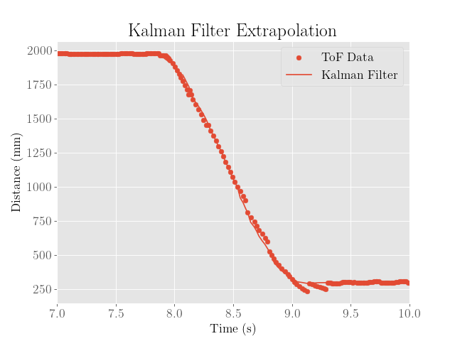
To test the filter’s capability to extrapolate, a simple sanity check in Python was performed, which simulated the extrapolation by skipping every eighth measurement.
After experimenting a bit with the filter, it was found that the system dynamics were better fit using the parameters $d = 0.0007$ and $h = 0.0002$, which seem to be closer to the original estimated parameter values:
 |
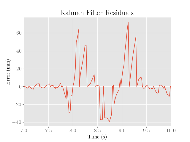 |
This ultimately worked fairly well, and resulted in filter estimates that closely matched the distance data, albeit with substantially more error than before:
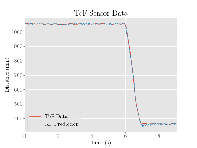
Note that because the datapoints are now being extrapolated with the Kalman filter, it is somewhat difficult to characterize the error without the actual distance measurement for reference.
One way to measure this might be to still collect these reference distance measurements when only the prediction step is being used.
However, collecting these measurements adds a significant amount of latency to the loop, which might not be representative of the performance of the filter when the measurement time budget and accuracy of the sensors is severely constrained.