Lab 4: IMU

The goal of this lab was to setup and characterize the Inertial Measurement Unit (IMU) sensor (ICM-20948) readings, which are used to provide information about the robots translational and angular motion.

Setup:

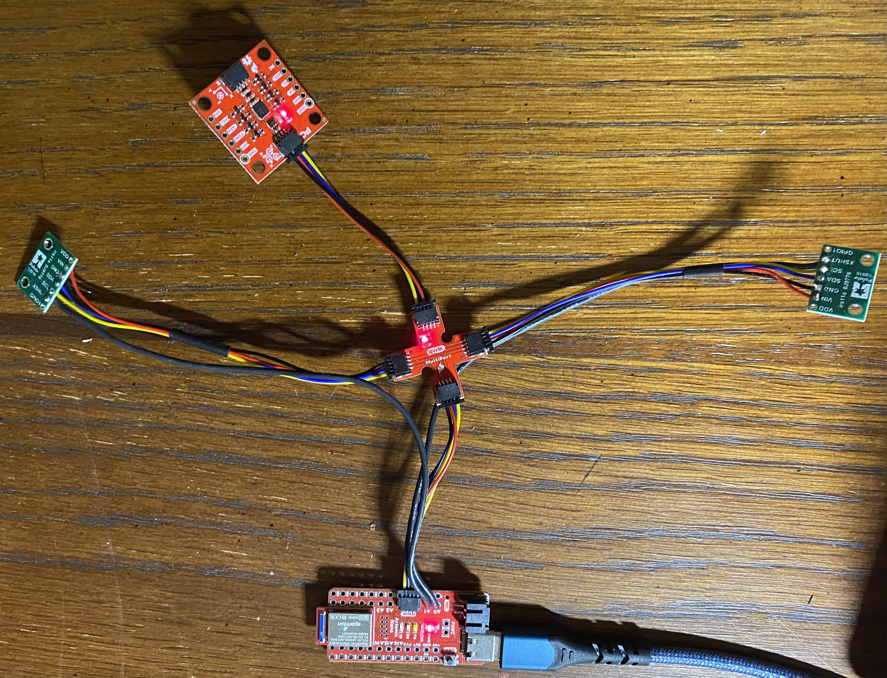
To begin, the IMU was wired to Artemis Nano using a 50 mm Quiic cable as shown below:

The IMU was then tested using the Basics script from the IMU Arduino Library, which was altered slightly to allow for easier visualizability through the Serial Plotter:

From the above video, we observe that in general, translational acceleration in each axis (x, y, and z) changes the accelerometer data, which is consistent with the data being measured in the units of gravitational acceleration.

Translating the board produced somewhat small changes in the accelerometer readings due to the near constant velocity of the board, but the changes in values became more apparent after jerking the board quickly up and down.

We also find that rotating the board to fixed angles changes the accelerometer data to fixed directions, which is due to the changing influence of the Earth’s gravitational acceleration on the sensor.

Furthermore, we also generally see that rotational movement of the board changes gyroscope data, which also agrees with the units of degrees per second.

This is a bit less noticeable due to how slowly the board was rotated, but it becomes more apparent after quickly shaking the board, which jerks the angles fast enough to get a visible change in the plotter.

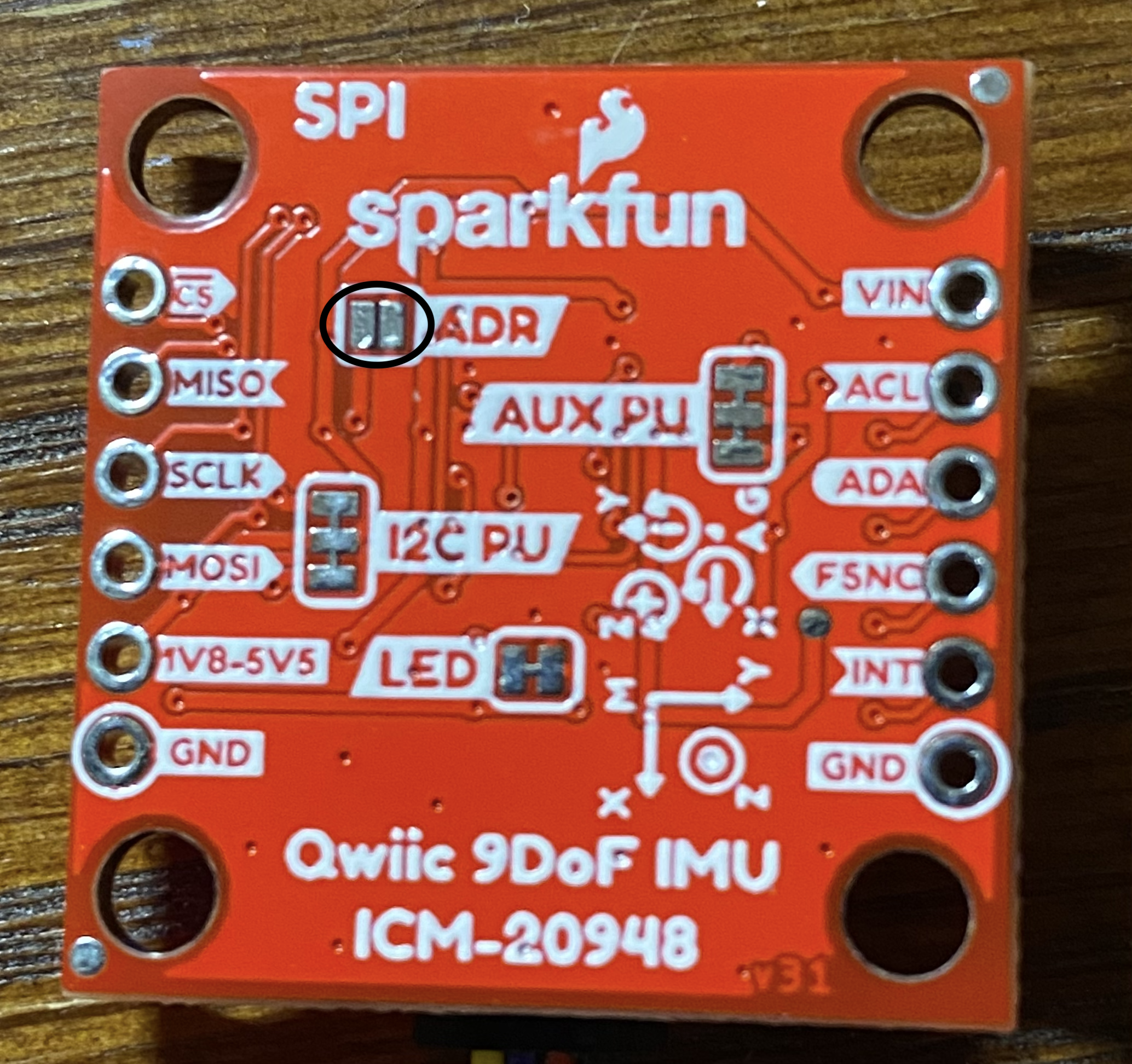
As an additional note, the script also required setting the constant AD0_VAL, which defined the last bit in the I2C address of the IMU. Since the ADR jumper on the board is not bridged, this value needed to be set to 1:

Accelerometer:

Next, the accelerometer was characterized by testing its accuracy in measuring pitch (\(\theta\)) and roll (\(\phi\)). This is easily accomplished by accounting for the influence of the Earth’s gravitational acceleration, which tells us that

\[\begin{align} a_x &= g\sin(\theta) \\ a_z &= g\cos(\theta) \\ \tan(\theta_a) &= \frac{a_x}{a_z} \\ \theta_a &= \arctan(\frac{a_x}{a_z}) \end{align}\]

Similarly, we know that

\[\begin{align} a_y &= g\sin(\phi) \\ a_z &= g\cos(\phi) \\ \tan(\phi_a) &= \frac{a_y}{a_z} \\ \phi_a &= \arctan(\frac{a_y}{a_z}) \end{align}\]

Translating these ideas into code gives us the following functions:

float getAPitch(ICM_20948_I2C *sensor){
  return atan2(sensor->accX()/sensor->accZ()) * 180/M_PI;
}

float getARoll(ICM_20948_I2C *sensor){
  return atan2(sensor->accY()/sensor->accZ()) * 180/M_PI;
}

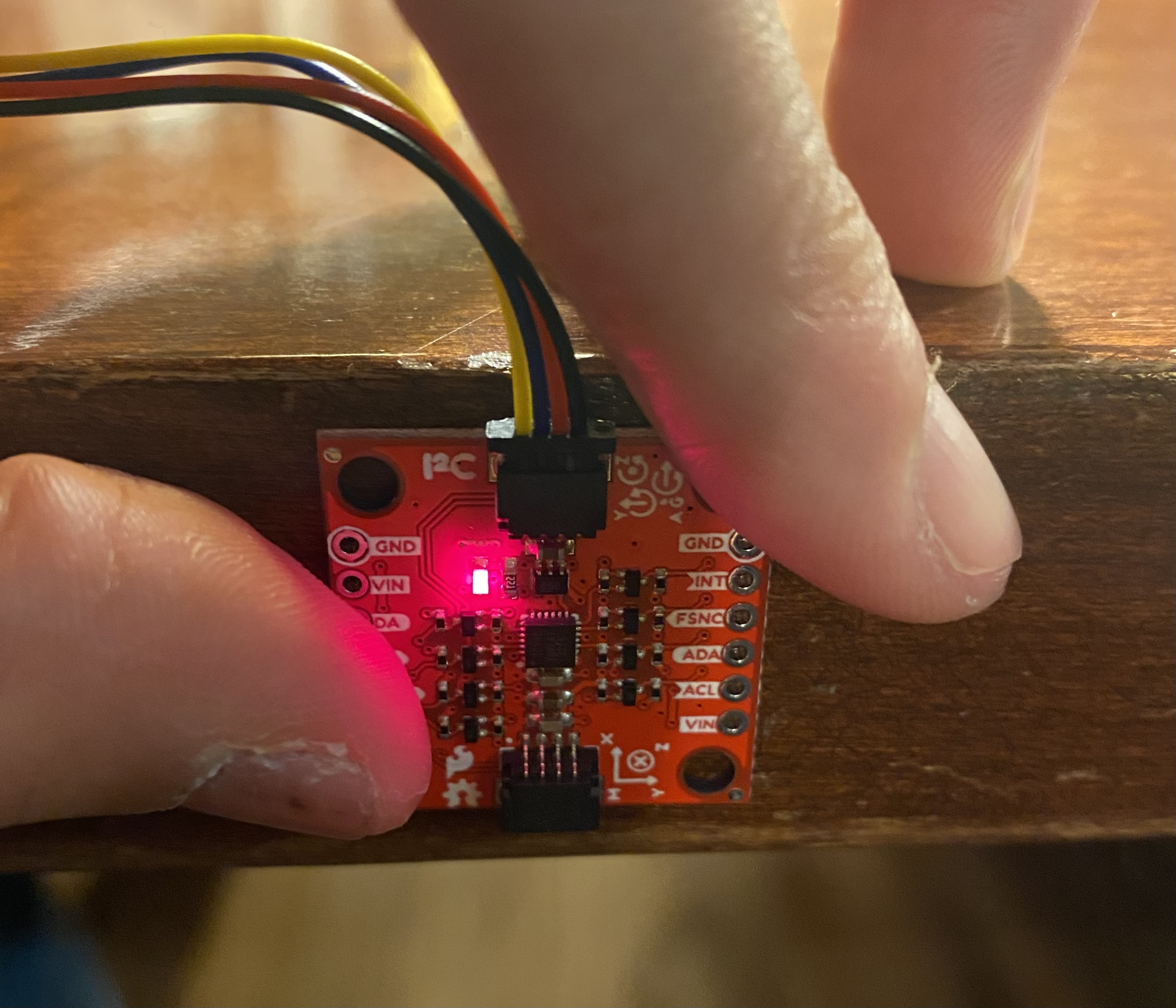
This was then tested against -90, 0, and 90 degrees pitch and roll, which were achieved by holding the IMU in various orientations against the surface of a table. An example for 90 degrees roll is shown below:

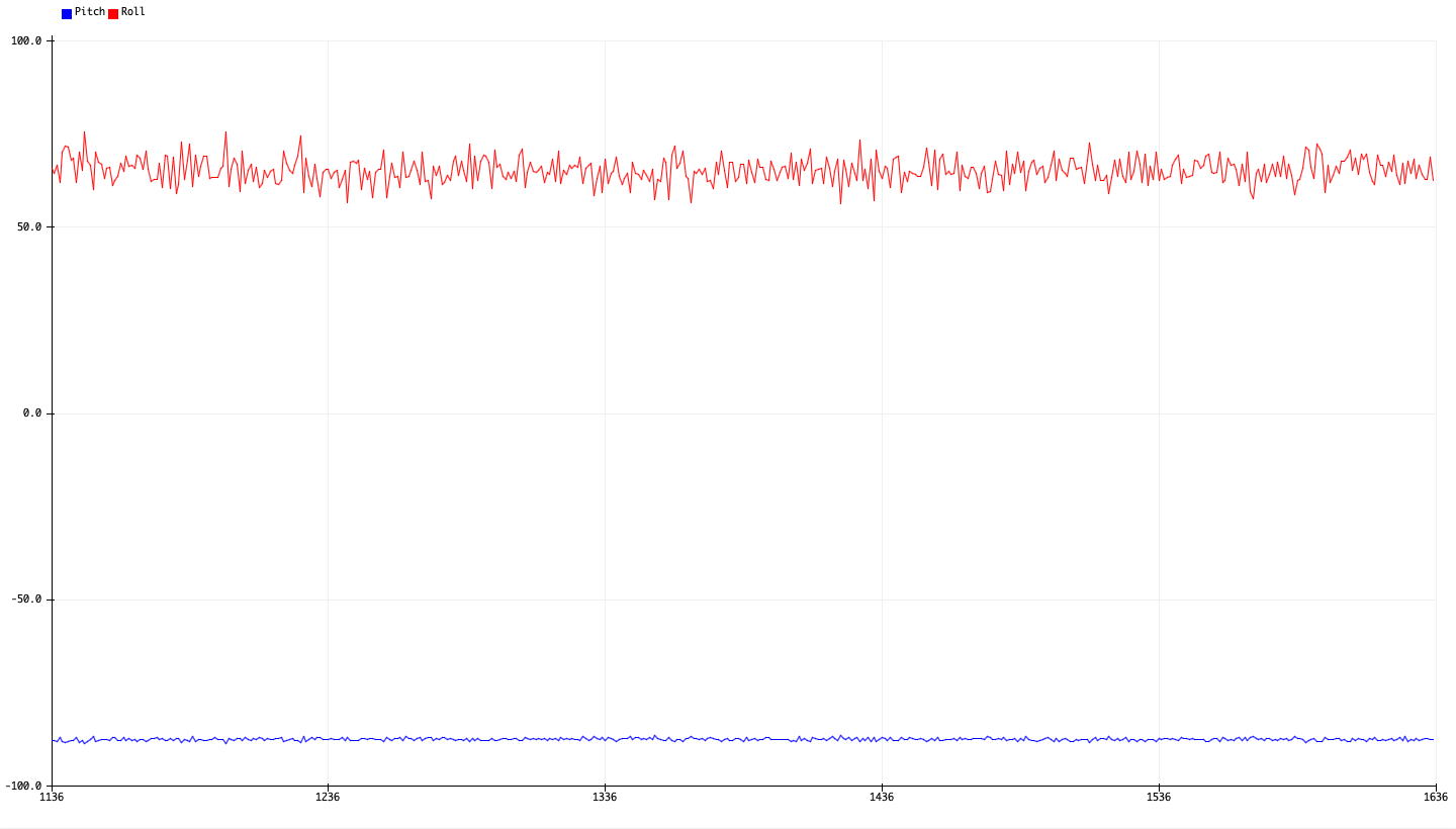
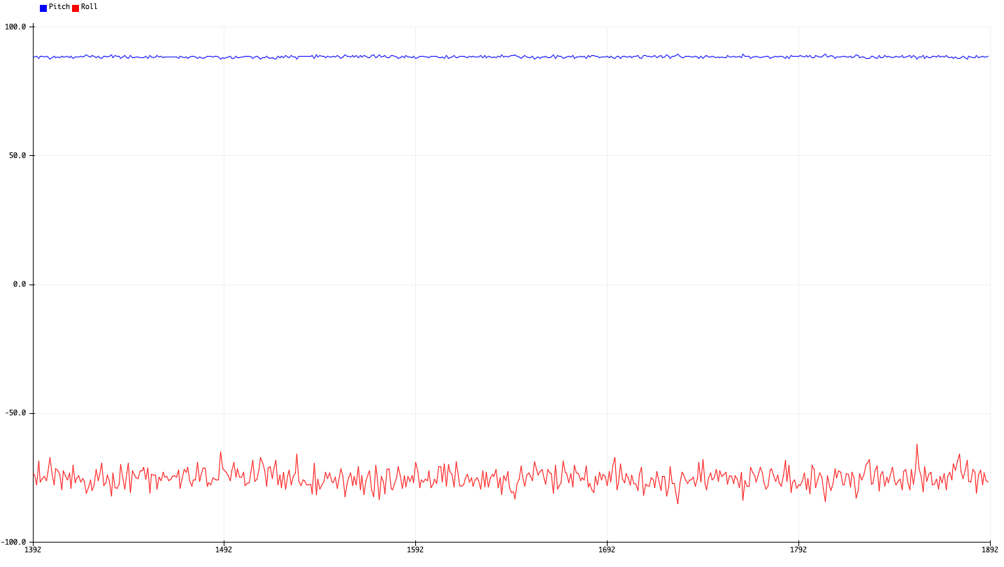
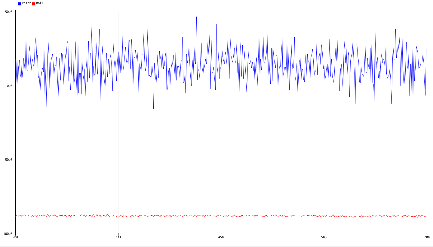
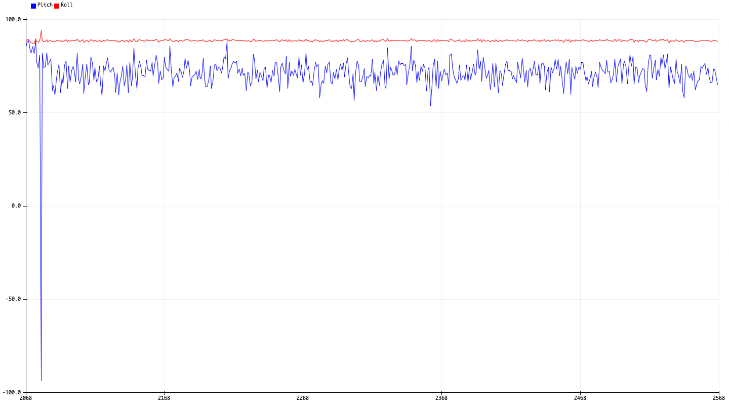
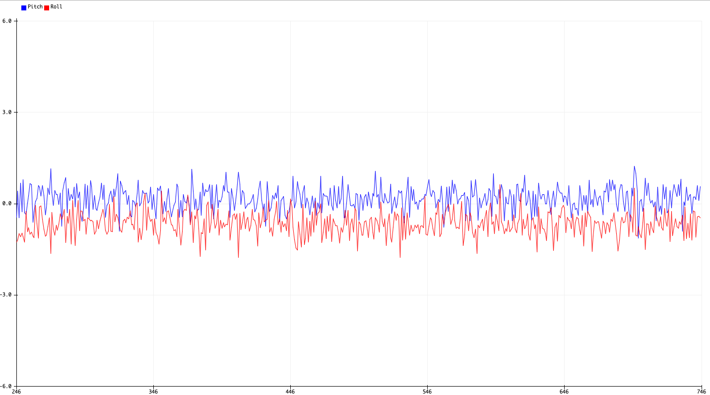
The following outputs were then obtained for -90, 90, and 0 degrees pitch and roll:

-90 Degrees Pitch	90 Degrees Pitch

-90 Degrees Roll	90 Degrees Roll

0 Degrees Pitch/Roll

Interestingly enough, we also see that although the roll and pitch should be near 0 when the other angle is 90 or -90 degrees, we actually observe very extreme fluctuations in these values.

One explanation for this is that the acceleration along the z-axis due to the influence of gravity becomes very small, making the calculated fraction \(a_x/a_z\) (or \(a_y/a_z\)) very sensitive to perturbations in measurements \(a_x\) and \(a_y\).

We would therefore expect the calculated angles to also vary very wildly, suggesting that this method is somewhat unwise to use when calculating angular orientations near \(\pm 90\) degrees in either pitch or roll.

The accuracy is then summarized below, where we compare the angles averaged over 100 measurements:

Actual Angle (Deg)	Average Measured Angle (Deg)		Absolute Error
	Pitch	Roll	Pitch	Roll
-90	-88.88	-88.27	1.12	1.73
0	0.36	-0.48	0.36	0.48
90	88.63	88.94	1.37	1.06

From here we observe that the measured angles are generally pretty accurate within about 1 or 2 degrees, which gets somewhat worse with large angles.

However, because the measured angles do not perfectly match the full -90 to 90 degree range, a more accurate estimate might be attained by performing a two-point calibration:

\[\begin{align} 90 - (-90) &= \alpha(\theta_{\text{measured},90} - \theta_{\text{measured},-90}) \end{align}\]

For future reference, the proportionality constants \(\alpha\) are listed below:

Angle	Two-Point Calibration Factor (\(\alpha\))
Pitch	1.0140
Roll	1.0157

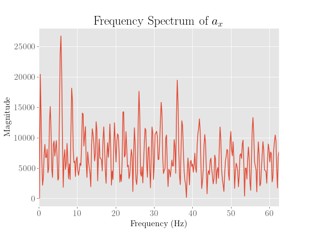
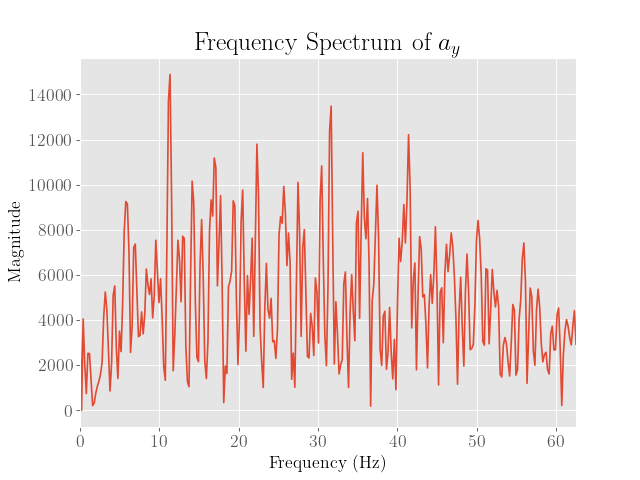
To analyze the noise in the acclerometer measurements, the following Python code was used to convert the stationary data sampled at 125 Hz to the frequency spectrum:

Fs = 125 
data = acc_mg[0][:]-np.mean(acc_mg[0][:])
N = len(data)
if N % 2 == 0:
    kvalues = np.arange(-N/2+1,N/2+1)
else:
    kvalues = np.arange(-(N-1)/2,(N-1)/2+1)

fvalues = kvalues*Fs/N
    
z = np.fft.fftshift(np.fft.fft(data))

Note that we subtract the DC component from the signals, which will produce a very large spike in the graph if left in. Furthermore, to test the sensitivity of the sensor to disturbances, the board was tapped several times to introduce impulses into the signal.

This then produced the following plots:

\(a_x\)	\(a_y\)	\(a_z\)

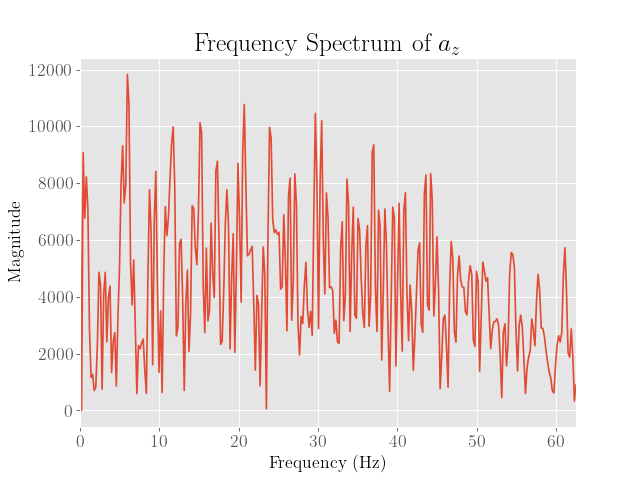From here we observe that the noise appears to peak at around 30 Hz, although this is more pronounced only for the y and z axes. We also note that the noise reaches this peak somewhat gradually, so a lower cutoff frequency may also prove to be beneficial.

We then consider a complementary low pass filter, which is characterized by

\[\begin{align} y_{LPF}[t+1] = \alpha y_{RAW}[t] + (1-\alpha) y_{LPF}[t] \end{align}\]

Here, we note that the parameter \(\alpha\) is given by

\[\begin{align} \alpha &= \frac{T_s}{T_s + 1/(2\pif_c)} \end{align}\]

Here, \(T_s\) is the sampling period, or the reciprocal of sampling frequency. Since we would like a cutoff frequency of 10 Hz at a sampling frequency of 100 Hz, we should choose $\alpha = 0.239$

From here we design the following complementary low pass filter, which has a cutoff frequency at 10 Hz:

float aLPFPitch = 0;
float getALPFPitch(ICM_20948_I2C *sensor){
  float alpha = 0.239;
  aLPFPitch = alpha*getAPitch(sensor) + (1-alpha)*aLPFPitch;
  return aLPFPitch;
}

float aLPFRoll = 0;
float getALPFRoll(ICM_20948_I2C *sensor){
  float alpha = 0.239;
  aLPFRoll = alpha*getARoll(sensor) + (1-alpha)*aLPFRoll;
  return aLPFRoll;
}

This yields the following output:

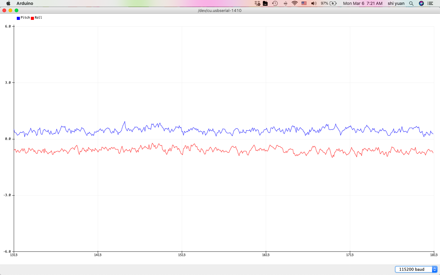
From here we observe that the fluctuations in the graph have been somewhat smoothed out, although there is still a noticeable amount of noise.

Gyroscope:

In order to fully estimate the angular orientation, we instead try an dead-reckoning approach with the gyroscope. To accomplish this, we note that

\[\begin{align} \theta_g(t) &= \theta_g(0) - \int g_x\;dt \\ \phi_g(t) &= \phi_g(0) - \int g_y\;dt \\ \psi_g(t) &= \psi_g(0) - \int g_z\;dt \end{align}\]

Note that since we use the right hand rule convention for positive angles, a negative sign is needed, as the gyroscope has a different sign convention.

However, because we are working with discrete samples in time, we use the following approximation:

\[\begin{align} \theta_g[t] &= \theta_g[t-1] - g_x\Delta t \\ \phi_g[t] &= \psi_g[t-1] - g_y\Delta t \\ \psi_g[t] &= \psi_g[t-1] - g_z\Delta t \end{align}\]

We then implement this into code:

float gPitch = 0;
int prevPitchTime = 0;
float getGPitch(ICM_20948_I2C *sensor){
  current = millis();
  float dt = (float) (current - prevPitchTime)/1000.0;
  prevPitchTime = current;
  gPitch = gPitch - dt*sensor->gyrY();
  return gPitch;
}

float gRoll = 0;
int prevRollTime = 0;
float getGRoll(ICM_20948_I2C *sensor){
  current = millis();
  float dt = (float) (millis() - prevRollTime)/1000.0;
  prevRollTime = current;
  gRoll = gRoll - dt*sensor->gyrX();
  return gRoll;
}

float gYaw = 0;
int prevYawTime = 0;
float getGYaw(ICM_20948_I2C *sensor){
  current = millis();
  float dt = (float) (millis() - prevYawTime)/1000.0;
  prevYawTime = current;
  gYaw = gYaw - dt*sensor->gyrZ();
  return gYaw;
}

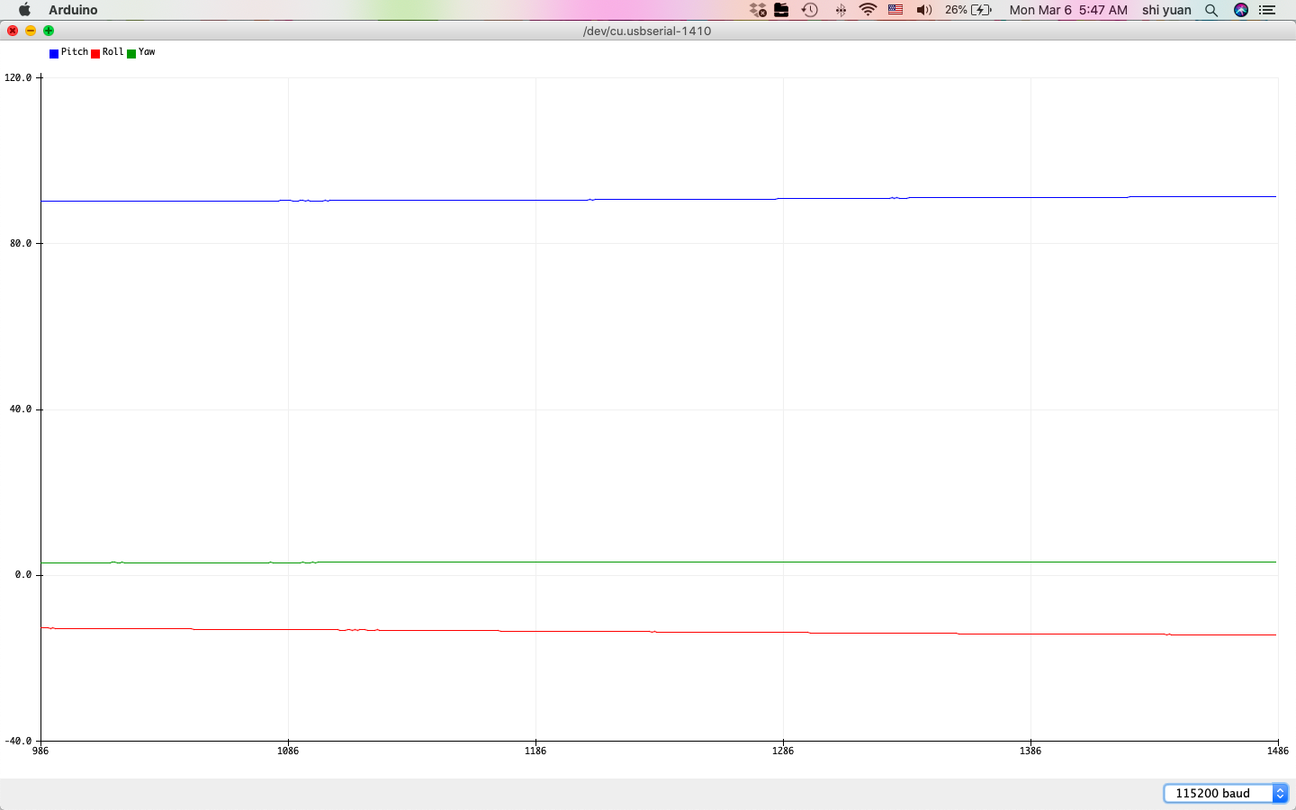
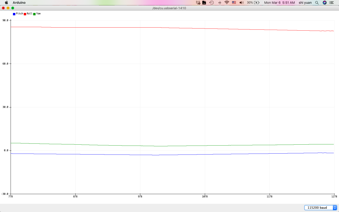
We then obtain the following plots of gyroscope readings at 90 degree angles for pitch, roll, and yaw:

Pitch	Roll	Yaw

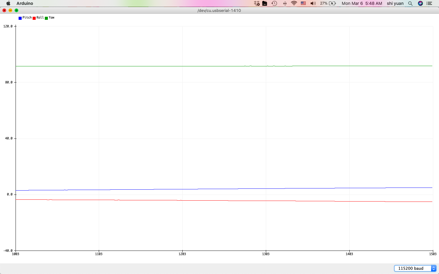After plotting these values, we see that the output angles are somewhat less noisy than their counterparts from the accelerometer calculations. Unlike the accelerometer measurements, we also observe that the angles no longer suffer from the large amounts of noise when the sensor is oriented at 90 degree angles, as the equations no longer suffer from numerical instability at these angles.

However, we do notice that the gyroscope readings sometimes result in a somewhat significant offset of around 10 degrees, as well as a significant drift in value, even when the board is stationary:

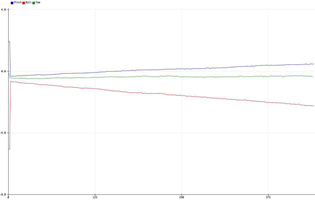As is usually the case with dead-reckoning methods, the errors from noise in the gyroscope readings and inaccuracies in the time interval measurements accrue over time. This then results in the calculated angles becoming increasingly more inaccurate with time, resulting in the observed drift.

Furthermore, we note that the drift does not lessen with slower sampling rates, and instead, the noise increases:

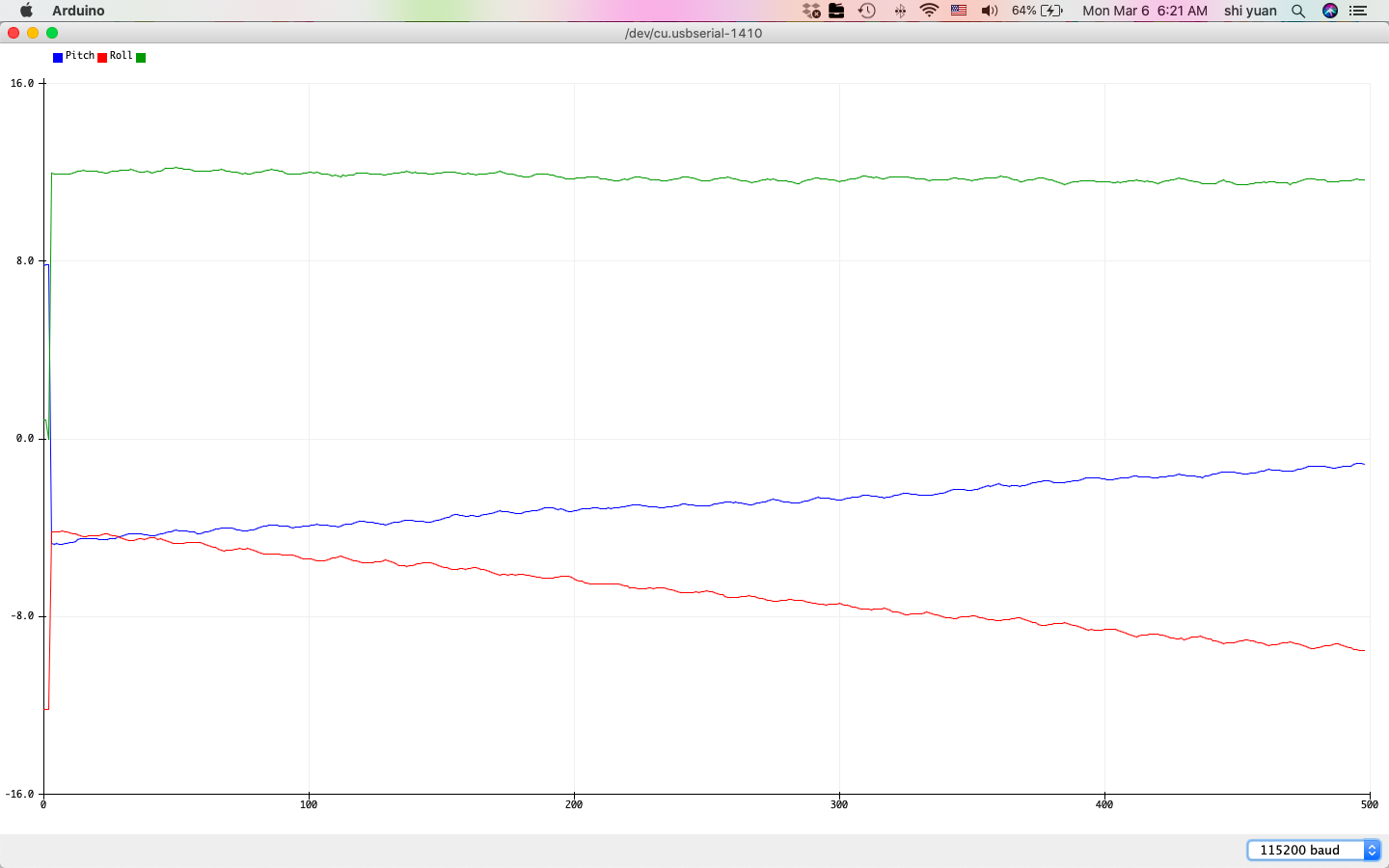Therefore to minimize drift, we simply sample without delay to maximize the sampling rate and hence the accuracy in measurements.

To improve the accuracy beyond the individual accelerometer and gyroscope measurements, we implement a complementary filter that combines both the angular estimates for pitch and roll from the (filtered) accelerometer and gyroscope:

\[\begin{align} \theta &= \alpha\theta_{a,LPF} + \theta_g(1-\alpha) \\ \phi &= \alpha\phi_{a,LPF} + \phi_g(1-\alpha) \end{align}\]

We then implement this in code via the following:

float getAGPitch(ICM_20948_I2C *sensor){
  float alpha = 0.5;
  return alpha*getALPFPitch(sensor) + (1-alpha)*getGPitch(sensor);
}

float getAGRoll(ICM_20948_I2C *sensor){
  float alpha = 0.5;
  return alpha*getALPFRoll(sensor) + (1-alpha)*getGRoll(sensor);
}

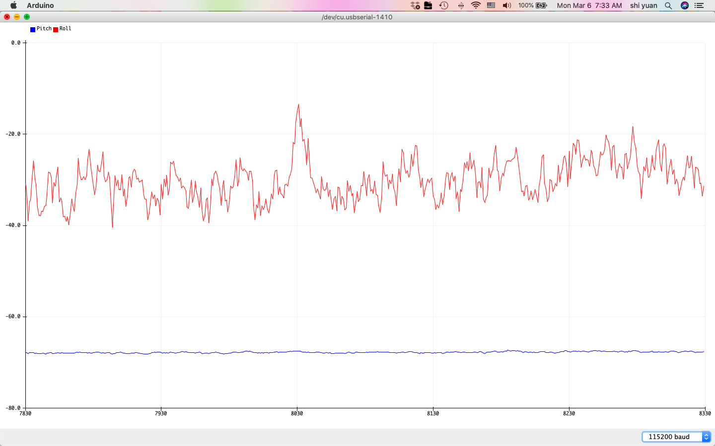
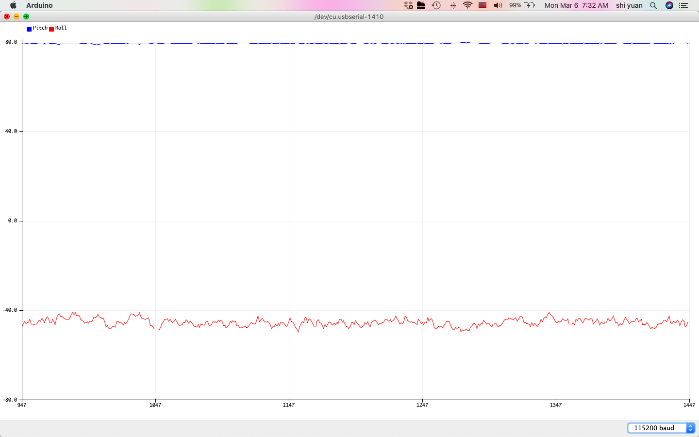
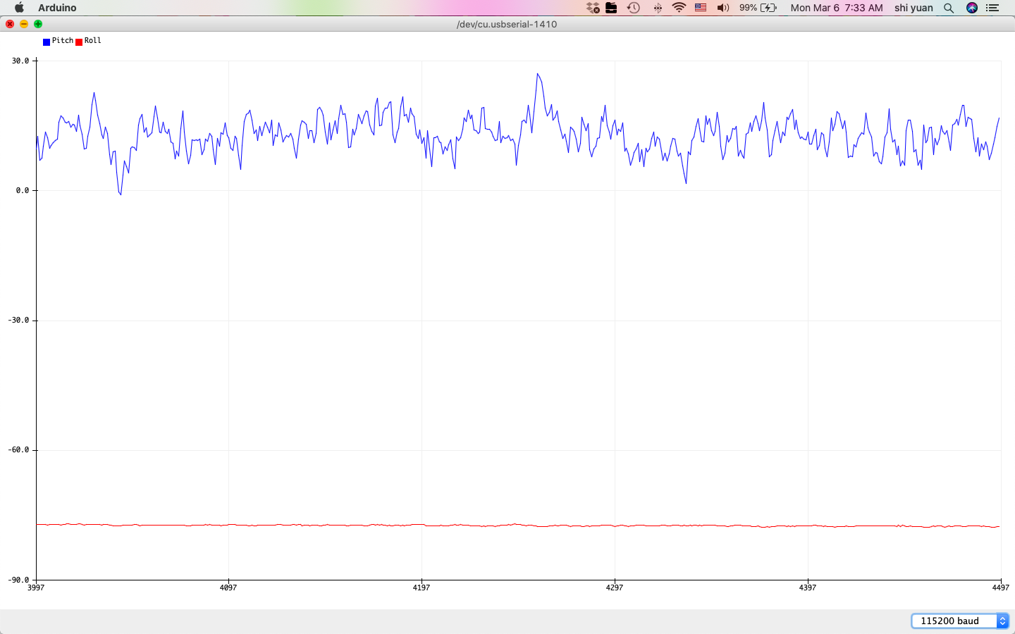
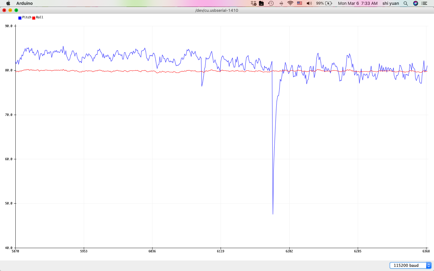
Here, we use $\alpha = 0.5$ to weigh the accelerometer readings more heavily to prevent drift. The resulting measurement is somewhat less noisier and less susceptible to drift and vibrations compared to the individual sensor readings:

-90 Degrees Filtered Pitch	90 Degrees Filtered Pitch

-90 Degrees Filtered Roll	90 Degrees Filtered Roll

0 Degrees Pitch/Roll

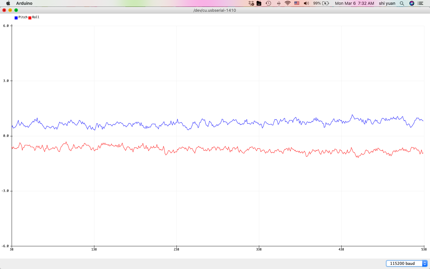While the sensor measurements produce smoother transitions in value and less drift, we also note that its effective range seems somewhat reduced, as the measurements near the ends of the range at -90 and 90 degrees are offset by about 10 degrees or more. The new effective range is no more than \((80 - 70)) = 150\) degrees for pitch and roll, where the new two-point calibration factor is then about \(\alpha = 1.2\).

Sample Data:

To speed up the sampling rate, we use the following loop, which samples data only when the sensor is ready:

#define MAX_SIZE 1000;
float ax[MAX_SIZE];
float ay[MAX_SIZE];
float az[MAX_SIZE];
float gx[MAX_SIZE];
float gy[MAX_SIZE];
float gz[MAX_SIZE];
int idx = 0;
int s = 0;

void loop()
{

  if (myICM.dataReady() && idx < WINDOW_SIZE)
  {
    Serial.println(millis()-s);
    s = millis();
    myICM.getAGMT();
    ax[idx] = (&myICM)->accX();
    ay[idx] = (&myICM)->accY();
    az[idx] = (&myICM)->accZ();
    gx[idx] = (&myICM)->gyrX();
    gy[idx] = (&myICM)->gyrX();
    gz[idx] = (&myICM)->gyrX();
    idx++;
  }
}

From here we find that the time between each measurement is roughly 2 to 3 milliseconds, indicating a sampling rate of about 333 to 500 Hz. Admittedly, printing the value to the Serial Monitor adds a small delay, meaning that this measurement is a slight overestimate.

To minimize the latency between sensor measurements, the Arduino code used to send the data was then split into two parts - one for collecting data and one for sending the data:

// Collect data
while(millis() - imu_prev < 5000){
  if (myICM.dataReady() && imu_idx < MAX_SIZE){
      myICM.getAGMT();
      imu_t[imu_idx] = int(millis());
      imu_ax[imu_idx] = (&myICM)->accX();
      imu_ay[imu_idx] = (&myICM)->accY();
      imu_az[imu_idx] = (&myICM)->accZ();
      imu_gx[imu_idx] = (&myICM)->gyrX();
      imu_gy[imu_idx] = (&myICM)->gyrY();
      imu_gz[imu_idx] = (&myICM)->gyrZ();
      imu_idx++;
  }
}
// Send data
for(int i = 0; i < imu_idx; i++){             
  tx_estring_value.append("T:");
  tx_estring_value.append(imu_t[i]); 
  tx_estring_value.append("|AX:");
  tx_estring_value.append(imu_ax[i]);
  tx_estring_value.append("|AY:");
  tx_estring_value.append(imu_ay[i]);
  tx_estring_value.append("|AZ:");
  tx_estring_value.append(imu_az[i]);
  tx_estring_value.append("|GX:");
  tx_estring_value.append(imu_gx[i]);
  tx_estring_value.append("|GY:");
  tx_estring_value.append(imu_gy[i]);
  tx_estring_value.append("|GZ:");
  tx_estring_value.append(imu_gz[i]);
  tx_characteristic_string.writeValue(tx_estring_value.c_str());
  tx_estring_value.clear();
}

To make post processing of the IMU data easier, we use separate 2D arrays for the accelerometer and gyroscope data, where data from each axis (x,y, and z) is stored in a separate row:

async def get_imu_5s_rapid(uuid,byte_array):
    global time_millis
    global acc_mg
    global gyr_dps
    global temp5s_str
    
    vecfloat = np.vectorize(lambda x: float(x[3::]))
    temp5s_str = ble.bytearray_to_string(byte_array)
    temp5s_list = temp5s_str.split("|")
    
    time = temp5s_list[0]

    a = temp5s_list[1:4] 
    g = temp5s_list[4:7] 

    time_millis.append(int(time[2::]))
    if len(acc_mg) == 0:
        acc_mg = np.reshape(vecfloat(a),(3,1))
    else:
        acc_mg = np.hstack((acc_mg,np.reshape(vecfloat(a),(3,1))))
    if len(gyr_dps) == 0:
        gyr_dps = np.reshape(vecfloat(g),(3,1))
    else:
        gyr_dps = np.hstack((gyr_dps,np.reshape(vecfloat(g),(3,1))))

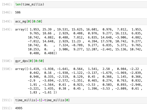
This yielded precisely 586 samples in 5 seconds:

We then integrate all sensors using the following Arduino code and notification handler, again using separate arrays to store data from different sensors:

// Collect data
while(millis() - ti_prev < 5000){
  if (myICM.dataReady() && distanceSensor1.checkForDataReady() && distanceSensor2.checkForDataReady() && ti_idx < MAX_SIZE)
  {
    myICM.getAGMT();
    t[ti_idx] = int(millis());
    ax[ti_idx] = (&myICM)->accX();
    ay[ti_idx] = (&myICM)->accY();
    az[ti_idx] = (&myICM)->accZ();
    gx[ti_idx] = (&myICM)->gyrX();
    gy[ti_idx] = (&myICM)->gyrY();
    gz[ti_idx] = (&myICM)->gyrZ();
    int distance1 = distanceSensor1.getDistance(); //Get the result of the measurement from the sensor
    int distance2 = distanceSensor2.getDistance(); //Get the result of the measurement from the sensor
    d1[ti_idx] = distance1;
    d2[ti_idx] = distance2;
    ti_idx++;
  }
}
// Send data
for(int i = 0; i < ti_idx; i++){             
    tx_estring_value.append("T:");
    tx_estring_value.append(t[i]); 
    tx_estring_value.append("|AX:");
    tx_estring_value.append(ax[i]);
    tx_estring_value.append("|AY:");
    tx_estring_value.append(ay[i]);
    tx_estring_value.append("|AZ:");
    tx_estring_value.append(az[i]);
    tx_estring_value.append("|GX:");
    tx_estring_value.append(gx[i]);
    tx_estring_value.append("|GY:");
    tx_estring_value.append(gy[i]);
    tx_estring_value.append("|GZ:");
    tx_estring_value.append(gz[i]);
    tx_estring_value.append("|D1:");
    tx_estring_value.append(d1[i]);
    tx_estring_value.append("|DZ:");
    tx_estring_value.append(d2[i]);        
    tx_characteristic_string.writeValue(tx_estring_value.c_str());
    tx_estring_value.clear();
}
break;

async def get_tof_imu_5s_rapid(uuid,byte_array):
    global time_millis
    global acc_mg
    global gyr_dps
    global depth1_mm
    global depth2_mm
    global temp5s_str
    
    vecfloat = np.vectorize(lambda x: float(x[3::]))
    temp5s_str = ble.bytearray_to_string(byte_array)
    temp5s_list = temp5s_str.split("|")
    
    time = temp5s_list[0]

    a = temp5s_list[1:4] 
    g = temp5s_list[4:7] 
    d = temp5s_list[7:9]
    time_millis.append(int(time[2::]))
    if len(acc_mg) == 0:
        acc_mg = np.reshape(vecfloat(a),(3,1))
    else:
        acc_mg = np.hstack((acc_mg,np.reshape(vecfloat(a),(3,1))))
    if len(gyr_dps) == 0:
        gyr_dps = np.reshape(vecfloat(g),(3,1))
    else:
        gyr_dps = np.hstack((gyr_dps,np.reshape(vecfloat(g),(3,1))))
    depth1_mm.append(int(d[0][3::]))
    depth2_mm.append(int(d[1][3::]))

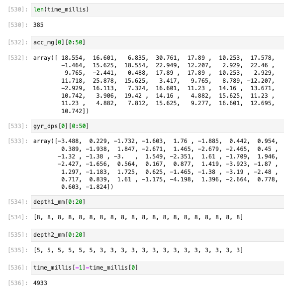
This code runs a bit slower compared to before, as it collects only 385 samples of timestamped data over a period of 5 seconds:

Considering that the combined payload of the ToF and IMU sensor data can get considerably large, the amount of memory allocated to the correpsonding sensor data arrays in the Artemis Nano must be carefully monitored.

To be more precise, each time-stamped sensor measurement consists of 3 float values from the accelerometer, 3 float values from the gyroscope, and 2 integer values from the time of flight sensors.

Given that single-precision float and integer values on the Artemis Nano require 4 bytes of storage for each value, each time-stamped set of sensor values requires preciesly 36 bytes of storage (including the time stamp).

Assuming a sampling rate of 150 Hz, we then find that the Artemis board can store about 65.99 seconds worth of sampled sensor data before running out of memory, meaning that the sensor data should be sent out every minute or so.

Battery:

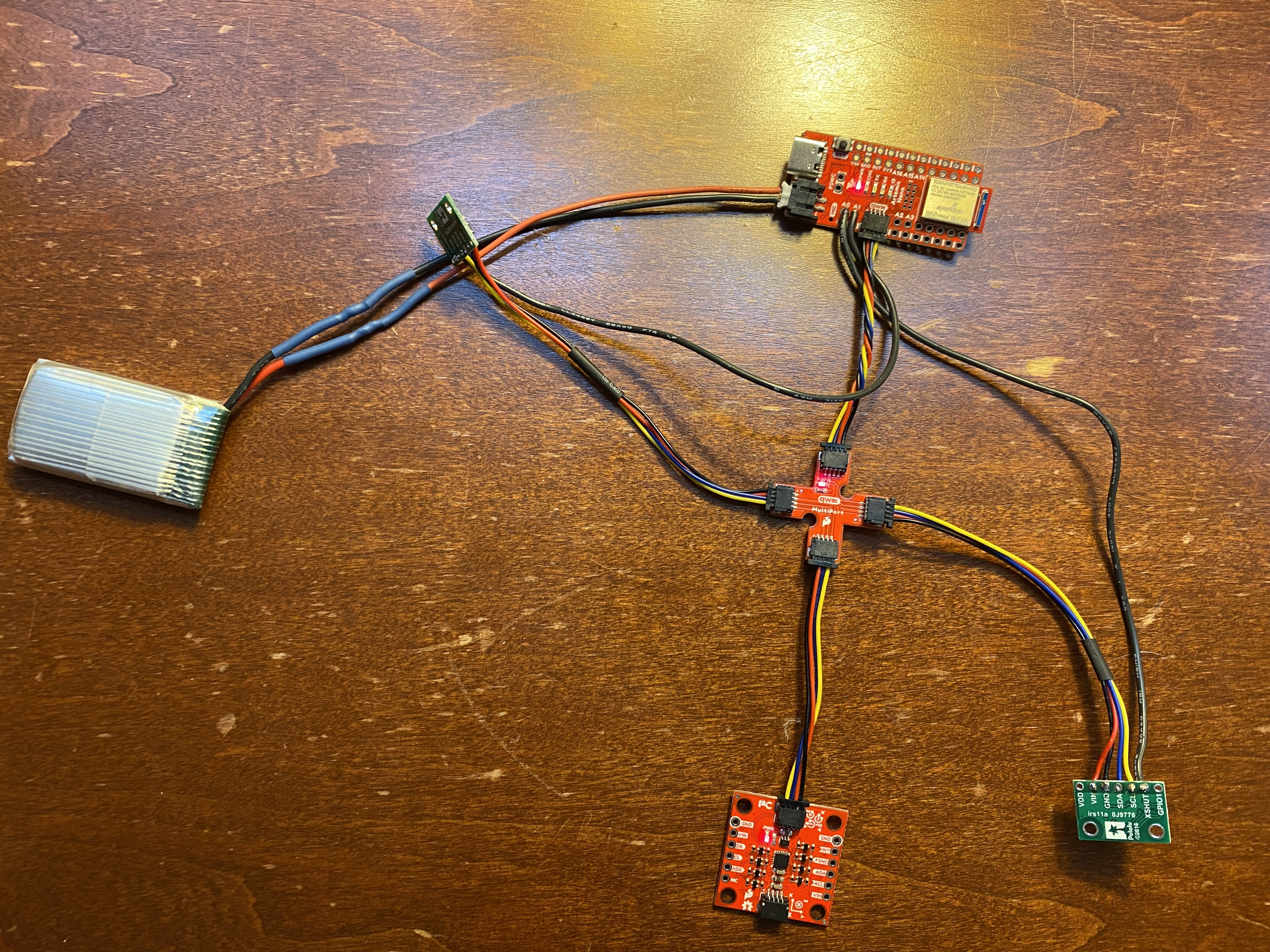
Next, we setup the batteries for the robot, which are divided into a 3.7 V 650 mAh LiPo battery for the Artemis Board and a 3.7 V 850 mAh LiPo battery to drive the motors.

The main advantages in setting up separate power supplies is to ensure a higher power output and lifetime for the motor power supply, which will draw much more current than the Artemis board needs to.Another benefit would be to possibly avoid ground loops and the possible addition of interference from the motors due to uneven loads on the power supply.

The battery setup is shown below:

RC Car:

After setting up the batteries, we then test out the car with a remote control to get a feel for its speed and manueverability on a laminate floor:

The Artemis board and sensor setup was then strapped to the car, where the sensor data was sent via Bluetooth during a simple stunt involving a skidding spin:

Plots of the collected sensor data are included below:

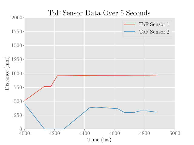
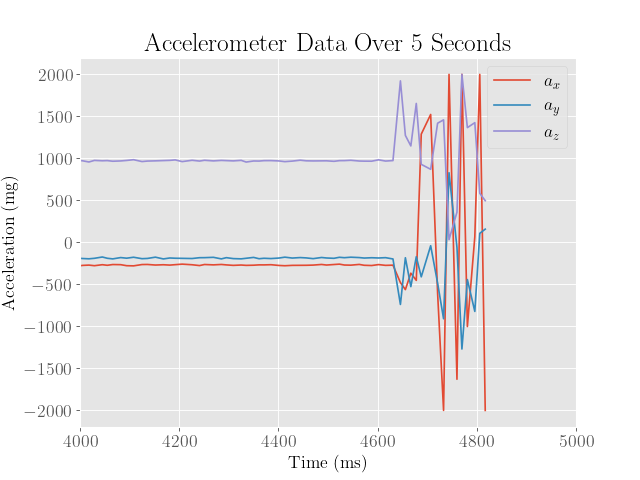
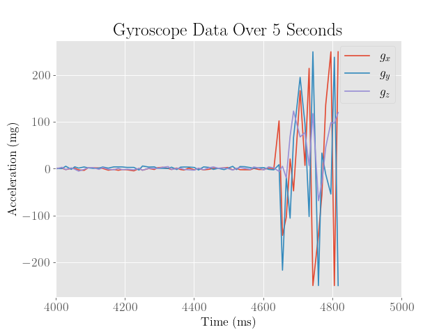
Because the sensor recording started a bit too early, most of the action really happens in the last second. We can see that the accelerometer and gyroscope data clearly indicate significant amounts of translational and angular movement. We also observe that the time of flight sensors indicate some change in distance to the surroundings, although this is somewhat less meaningful since the sensors were not securely mounted onto the robot.