Lab 12: Path Planning and Execution
For the final lab, the goal was to utilize the algorithms and tools developed in previous labs to compute a motion planning task in the lab maze, where the robot would navigate to 9 marked waypoints.
Waypoints
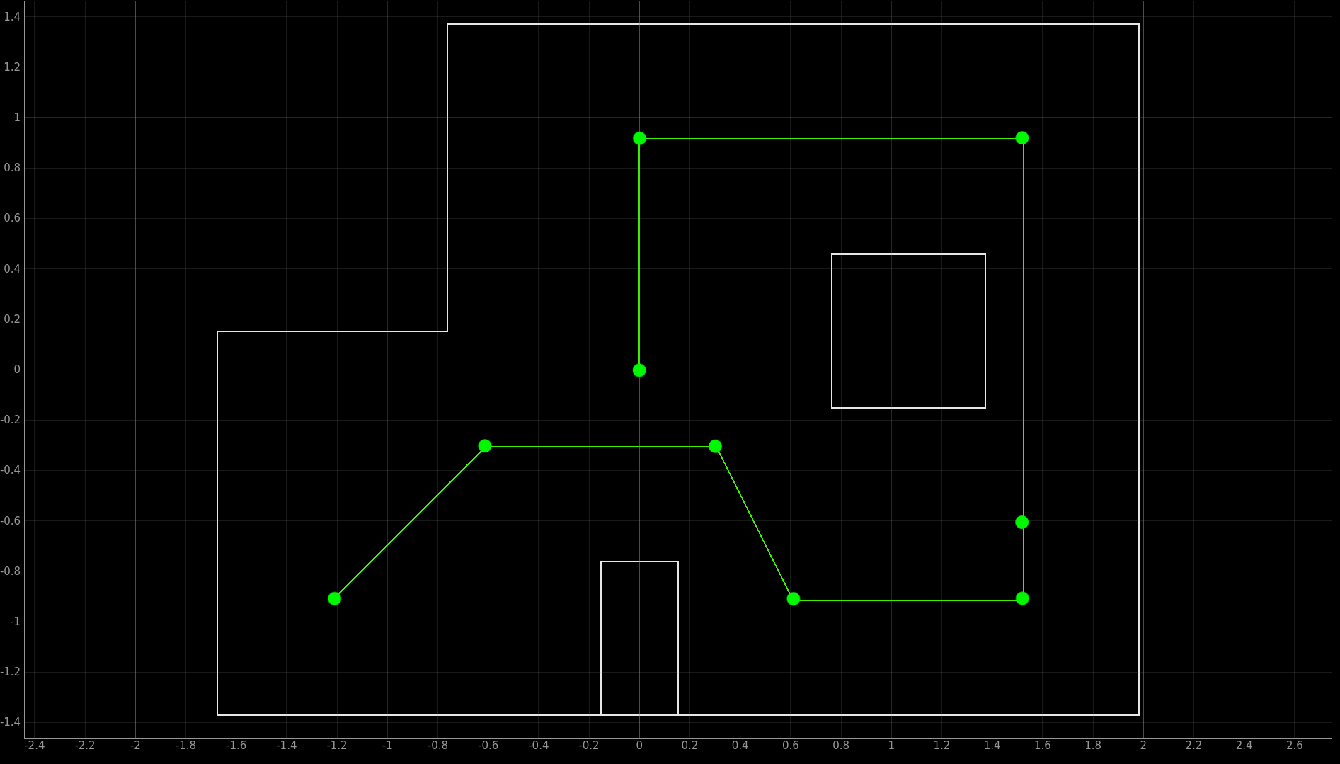
We first provide a list of the waypoints:
1. (-4, -3)
2. (-2, -1)
3. (1, -1)
4. (2, -3)
5. (5, -3)
6. (5, -2)
7. (5, 3)
8. (0, 3)
9. (0, 0)
These can be visualized with the following image:

Path Planning
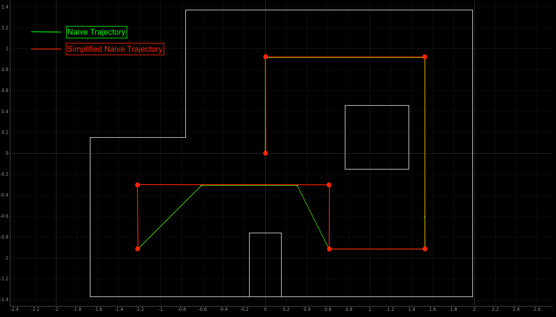
For this lab, the first approach was to implement a naive trajectory consisting of only forward movements and pure rotations.
The robot would then reach the waypoints via PID controllers on the distance to the walls and the yaw from the IMU.
To simplify the trajectory even further, we use an idea borrowed from Ryan Chan (class of 2022 offering) to ensure only 90 degree rotations are required:
1. (-4, -3)
2. (-4, -1)
3. (2, -1)
4. (2, -3)
5. (5, -3)
6. (5, 3)
7. (0, 3)
8. (0, 0)

A slightly more subtle point about this approach is that the ToF sensors are not capable of measuring distances past roughly 1.8 meters, the sensor will outputs zeros past this point (even in the “long” mode). This seems to contradict the datasheet, and is probably a consequence of setting a measurement time budget that is too short. However, extending the time budget would mean a longer sampling time and less accurate control, so this option wasn’t explored for this lab to make the solution slightly more robust.
To work around the limited sensor range, the robot was programmed to turn facing the closest wall, and then back up to the PID setpoint. Despite this, the robot will still need to back up past the maximum sensor range. While one option would be to simply perform a 180 degree rotation so that it would face a closer wall, this was somewhat more risky since the robot’s orientation control was pretty unreliable.
Since these distances were only about a foot outside the maximum sensor range, the solution was to simply add a short open loop control boost to the motor values for about 0.2 seconds.
To program the simplified trajectory on the robot, this required essentially programming every single action.
A different way to program the trajectory that could better scale with large numbers of waypoints would be to write a script to calculate the exact angle or distance setpoints to reach the next waypoint.
Below we include a list of the setpoints and actions used to complete the trajectory:
1. Distance Setpoint:  457  mm
2. Angular Setpoint:   90   deg
3. Distance Setpoint:  1676 mm + Open Loop Boost
4. Angular Setpoint;   180  deg
5. Distance Setpoint:  457  mm
6. Angular Setpoint : -90   deg
7. Distance Setpoint:  457  mm
8. Angular Setpoint:  -180  deg
9. Distance Setpoint:  1800 mm + Open Loop Boost
10. Angular Setpoint: -90   deg
11. Distance Setpoint: 1676 mm + Open Loop Boost
12. Angular Setpoint:  0    deg
13. Distance Setpoint: 1676 mm
Note that we take the initial angular orientation as 0 degrees, and that we actually subtract a small offset of about 70mm to each of the setpoints to ensure that the center of the robot reaches the setpoint.
After testing this out on the real maze, the robot successfully passes through all the waypoints:
In hindsight, this approach was too optimistic about the degree of control the robot had over orientation, as the turns were very inconsistent in accuracy. The true rate of success of this approach was probably no greater than 1 out of every 20 runs. This was partially because the yaw readings were pretty unreliable, and would drastically change upon moving too quickly or from shaking.
In a sense, using PID control on the distance from the walls is similar to using a localization algorithm, since it uses distance measurements and knowledge about the map to guide the robot to each waypoints. It also might potentially be faster, since it cuts out the observation loops needed for estimating the pose.
The main difference is that the localization algorithm is also capable to discerning the exact angular pose of the robot, whereas simple PID control relies on the measurements from the IMU to get the robot’s orientation.
The other disadvantage with this approach is that it makes no effort to correct the orientation of the robot while driving forward, which puts it at risk to collide with walls. This was especially a problem with traversing long distances, since the robot would deviate more from the desired course with even a slightly incorrect angular pose.
Absolute Orientation
As a small aside, the angular orientation was calculated by accessing a Digital Motion Processor (DMP) included with the ICM-20948 IMU. In short, the DMP was a digital signal processor specialized for accelerating sensor fusion algorithms for the IMU, and would output quaternions for orientation.
This ideally would not only make the code for calculating the angular orientation of the robot more simple, but also potentially read out more accurate orientations, as the DMP incorporates even the magnetometer readings and already includes filtering algorithms to minimize measurement noise.
These features were easily accessible from the Sparkfun ICM-20948 Arduino library, and using the DMP readings required a small snippet of code to initialize the device, as well as a couple of lines to read out and convert the quaternion data into the robot’s angular pose.
To initialize the DMP we use the following in the setup function:
bool success = true;
success &= (myICM.initializeDMP() == ICM_20948_Stat_Ok);
success &= (myICM.enableDMPSensor(INV_ICM20948_SENSOR_ORIENTATION) == ICM_20948_Stat_Ok);
success &= (myICM.setDMPODRrate(DMP_ODR_Reg_Quat9, 0) == ICM_20948_Stat_Ok);
success &= (myICM.enableFIFO() == ICM_20948_Stat_Ok);
success &= (myICM.enableDMP() == ICM_20948_Stat_Ok);
success &= (myICM.resetDMP() == ICM_20948_Stat_Ok);
success &= (myICM.resetFIFO() == ICM_20948_Stat_Ok);
To readout the data, we include the following inside the main loop:
icm_20948_DMP_data_t data;
myICM.readDMPdataFromFIFO(&data);
Finally, to ensure that the sensor readings are valid, the following check was included:
(myICM.status == ICM_20948_Stat_Ok) || (myICM.status == ICM_20948_Stat_FIFOMoreDataAvail)
To actually convert the quaternion data into the yaw of the robot, this required math that might be hard to follow. Quaternions are basically 4 dimensional complex numbers, so the actual meaning of the data is not very intuitive to begin with. However, it sufficed to simply copy from the library examples:
double q1 = ((double)data.Quat9.Data.Q1) / 1073741824.0;
double q2 = ((double)data.Quat9.Data.Q2) / 1073741824.0;
double q3 = ((double)data.Quat9.Data.Q3) / 1073741824.0;
double q0 = sqrt(1.0 - ((q1 * q1) + (q2 * q2) + (q3 * q3)));
yaw[idx] = getYaw(q0,q1,q2,q3);

double getYaw(double q0, double q1, double q2, double q3) {
    double q2sqr = q2 * q2;
    double t3 = +2.0 * (q0 * q3 + q1 * q2);
    double t4 = +1.0 - 2.0 * (q2sqr + q3 * q3);
    return atan2(t3, t4) * 180.0 / PI;
}
An additional subtlety with using the DMP is that it resets all biases used to calibrate the IMU sensor readings upon powering off, as the device does not have any onboard memory. To ensure that the device is properly calibrated, the sensor needs to be rotated on each of the 6 axes for about 2 minutes to get the right biases.
While this might seem inconvenient, the DMP also will figure out the absolute orientation of the robot in the process, which saves the effort of finding the right rotation matrices to transform the data.
Furthermore, the biases can be saved into the flash memory of the Artemis microcontroller, which can then be loaded into the registers of the DMP upon initializing.
To read the baises, the following was included in the setup function:
EEPROM.init();

biasStore store;

EEPROM.get(0, store); // Read existing EEPROM, starting at address 0
if (isBiasStoreValid(&store))
{
    Serial.println(F("Bias data in EEPROM is valid. Restoring it..."));
    success &= (myICM.setBiasGyroX(store.biasGyroX) == ICM_20948_Stat_Ok);
    success &= (myICM.setBiasGyroY(store.biasGyroY) == ICM_20948_Stat_Ok);
    success &= (myICM.setBiasGyroZ(store.biasGyroZ) == ICM_20948_Stat_Ok);
    success &= (myICM.setBiasAccelX(store.biasAccelX) == ICM_20948_Stat_Ok);
    success &= (myICM.setBiasAccelY(store.biasAccelY) == ICM_20948_Stat_Ok);
    success &= (myICM.setBiasAccelZ(store.biasAccelZ) == ICM_20948_Stat_Ok);
    success &= (myICM.setBiasCPassX(store.biasCPassX) == ICM_20948_Stat_Ok);
    success &= (myICM.setBiasCPassY(store.biasCPassY) == ICM_20948_Stat_Ok);
    success &= (myICM.setBiasCPassZ(store.biasCPassZ) == ICM_20948_Stat_Ok);
}
To store biases upon disconnecting and shutting off, we include the following:
bool success = (myICM.getBiasGyroX(&store.biasGyroX) == ICM_20948_Stat_Ok);
success &= (myICM.getBiasGyroY(&store.biasGyroY) == ICM_20948_Stat_Ok);
success &= (myICM.getBiasGyroZ(&store.biasGyroZ) == ICM_20948_Stat_Ok);
success &= (myICM.getBiasAccelX(&store.biasAccelX) == ICM_20948_Stat_Ok);
success &= (myICM.getBiasAccelY(&store.biasAccelY) == ICM_20948_Stat_Ok);
success &= (myICM.getBiasAccelZ(&store.biasAccelZ) == ICM_20948_Stat_Ok);
success &= (myICM.getBiasCPassX(&store.biasCPassX) == ICM_20948_Stat_Ok);
success &= (myICM.getBiasCPassY(&store.biasCPassY) == ICM_20948_Stat_Ok);
success &= (myICM.getBiasCPassZ(&store.biasCPassZ) == ICM_20948_Stat_Ok);

updateBiasStoreSum(&store);

if (success)
{
    EEPROM.put(0, store);
    EEPROM.get(0, store);
}
This ultimately seems to give pretty robust orientation readings that will keep track of the angle within a few degrees, even after violently shaking the robot.
To show that this actually works, we include an video of the Serial plotter readings after making 90 degree rotations:
Although it might be hard to see the exact yaw values, the rotations roughly change the yaw values by somewhere between 90 to 100 degrees each turn with virtually no noise whatsoever, suggesting that the data is both quite precise and accurate. It also avoids drift problems from the gyroscope to some extent, as the values seem to stabilize after a while.
It is admittedly hard to say what exactly the sensor fusion algorithms are doing, since the DMP is essentially a black box.This obviously also isn’t the most rigorous test of the DMP, and it is definitely worth further investigating the error and biases of the yaw readings using this approach.
In hindsight, calculating orientation with a magnetometer may not be a good idea in the first place, since the IMU was placed very closely to the motors. The magnetic field interference certainly isn’t i.i.d. Gaussian, so it wouldn’t be surprising if that made the orientation readings inaccurate. There were certainly many occasions where the yaw readings became completely meaningless and the robot would lose control over orientation.
To mitigate issues with interference, periodic pauses were inserted between each movement, and the yaw control was repeated with refining tolerances to hopefully correct the orientation if the yaw values became more accurate over an idle period. This seemed to help some of the time, but it was still admittedly pretty unreliable. The accuracy of a PID control based approach depends almost entirely on the level of orientation control, so this made getting a successful run pretty difficult overall.
A better solution may have been to simply use a localization algorithm, and possible use the orientation readings from the IMU to correct mistakes. Since the IMU would inevitably give inaccurate readings, it might be better to discount the confidence in the IMU readings. A more interesting approach would be to use the magnetometer from the IMU as a motor encoder, and to hopefully improve the prediction step of the Bayes Filter this way.
Finally, another approach that would be interesting to try would be to attempt some form of optimal control with LQR and somehow integrate that with path planning, but this would only really work if the robot had a better way to localize itself in the map.