Lab 11: Localization on the Real Robot

In this lab, the grid localization filter developed in Lab 10 was carried over from the simulator to the real robot.

Simulation

To begin, we include a brief test of the filter under the simulation, Note that in order to improve the performance of the filter, we use the following vectorizations of the filter in the localization_extras.py file:

def compute_control(self, cur_pose, prev_pose):
    total_rot =  (180/np.pi)*np.arctan2((cur_pose[:,1] - prev_pose[:,1]), 
                                        (cur_pose[:,0]-prev_pose[:,0]))
    delta_rot_1 = self.mapper.normalize_angle(total_rot - prev_pose[:,2])
    delta_trans = np.linalg.norm(cur_pose[:,0:2]-prev_pose[:,0:2],axis = 1)
    delta_rot_2 = self.mapper.normalize_angle(cur_pose[:,2] - total_rot)
    return delta_rot_1, delta_trans, delta_rot_2

def odom_motion_model(self, cur_pose, prev_pose, u):
    delta_rot_1, delta_trans, delta_rot_2 = self.compute_control(cur_pose,prev_pose)
    rot_1_prob = self.gaussian(delta_rot_1,u[0],self.odom_rot_sigma)
    trans_prob = self.gaussian(delta_trans,u[1],self.odom_trans_sigma)
    rot_2_prob = self.gaussian(delta_rot_2,u[2],self.odom_rot_sigma)
    prob = rot_1_prob * trans_prob * rot_2_prob
    return prob

def prediction_step(self, cur_odom, prev_odom):
    u = self.compute_control(np.array([cur_odom,]), np.array([prev_odom,]))
    bel_array = np.ravel(self.bel,order = 'C')
    idx = np.nonzero(bel_array > 0.000001)
    prob = self.odom_motion_model(self.mapper.get_cur_poses(idx),self.mapper.get_prev_poses(idx),u)
    prob_array = np.reshape(prob,(self.mapper.total,len(idx[0])),order = 'C')
    predictions = np.dot(prob_array,bel_array[idx])
    self.bel_bar = np.reshape(predictions,self.bel.shape,order = 'C')
    self.bel_bar[self.mapper.get_forbidden()] = 0
    eta = 1/(np.sum(self.bel_bar))
    self.bel_bar = self.bel_bar*eta
        
def sensor_model(self,obs):
    obs_range_data = np.tile(np.squeeze(self.obs_range_data),(self.mapper.total,1))
    prob_array = self.gaussian(obs_range_data,obs,self.sensor_sigma)    
    return prob_array
        
def update_step(self):
    self.bel = deepcopy(self.bel_bar)
    obs_array = np.reshape(self.mapper.get_full_views(),(self.mapper.total,self.mapper.OBS_PER_CELL),order = 'C')
    prob_array = self.sensor_model(obs_array)
    updates = np.prod(prob_array,axis = 1)
    self.bel = np.reshape(updates,self.bel_bar.shape,order = 'C')*self.bel
    eta = 1/(np.sum(self.bel))
    self.bel = self.bel * eta

def normalize_angle(self, a):
    return a - (np.floor((a + 180)/360))*360

The key improvements in the efficiency of the code mainly included broadcasting the likelihood computations in odom_motion_model() and compute_control() over arrays of multiple poses. This then allowed for parallel processing of every pose combination, which completely removed the need for nested for loops.

Although the sensor_model() and update_step() functions were relatively easy to vectorize and test, the prediction_step() was particularly challenging and required several reshaping commands to make processing easier.

Another feature of the rewritten functions is the inclusion of checks for when the previous timestep’s belief is negligible, which then prompts the function to discard these entries in the final calculation of the likelihoods. This was implementing by slicing out the irrelevant entries:

def get_cur_poses(self,idx):
    mask = np.zeros((self.total,), dtype=bool)
    mask[idx] = 1
    return self.cur_poses[np.repeat(mask,self.total)]
    
def get_prev_poses(self,idx):
    mask = np.zeros((self.total,), dtype=bool)
    mask[idx] = 1
    return self.prev_poses[np.repeat(mask,self.total)]

Finally, we also note that the prediction step also accounts for forbidden regions of the map, and sets the corresponding beliefs to zero for those locations:

def get_forbidden(self):
    val_x = np.reshape(self.poses[:,0], self.cells.shape,order = 'C')
    val_y = np.reshape(self.poses[:,1], self.cells.shape,order = 'C')
    idx = np.zeros(self.cells.shape, dtype = bool)
    # Box 1
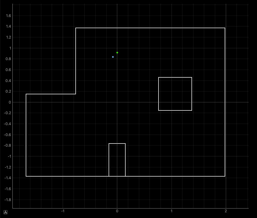
    idx[(val_x>=-0.152) & (val_x<=0.152) & (val_y >= -1.372) & (val_y <= -0.762)] = 1
    # Box 2
    idx[(val_x>=0.762) & (val_x<=1.372) & (val_y >= -0.153) & (val_y <= 0.458)] = 1
    # Walls
    idx[(val_x<=-0.762) & (val_y >= -0.152)] = 1
    return idx

Granted, these improvements only provide very marginal improvements to the filter’s accuracy, since the disturbances to the robot’s motion are quite large. Instead, the update step seems to provide the most accurate estimates of the pose, but it certainly wouldn’t hurt to gather more information from the odometry of the robot.

To show that this actually works, we run this in the simulator:

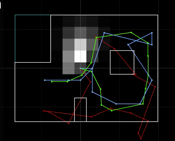
Observation Loop

Next, we proceed to implement an observation loop that commands the robot to take ToF measurements while rotating a full 360 degrees, which will be crucial to collecting measurements for the update step of the Bayes Filter.

To implement this loop on the robot, a PID controller was used to control the yaw velocity, which would be stopped once the robot had completed a full 360 degree displacement in yaw.

case OBS_LOOP:
    if (!loop_started){
      yaw_setpoint = yaw[previdx];
      idx = 0;
      disp = 0;
      loop_started = true;
    }
    float phi;
    phi = yaw[previdx] - yaw_setpoint;
    yaw_setpoint = yaw[previdx];
    if (phi >= 180) {
      phi -= 360;
    } 
    if (phi < -180) {
      phi += 360;
    }  
    disp += phi;
    SERIAL_PORT.println(disp);

    if(abs(disp) <= 360)
    {
      yaw_vel_control();
    }
    else
    {
      analogWrite(A15,255);
      analogWrite(A16,255);
      analogWrite(4,255);
      analogWrite(A5,255);
      send_obs(360);
    }
    break;

During the rotation, distance measurements are collected as fast as possible, where a fixed number of measurements is sent to the laptop that is safely below the typical number of measurements completed in a single loop. Each value of distance is then stamped with a corresponding yaw value for post-processing purposes.

void send_obs(int size)
{
    tx_estring_value.clear();
    
    // Send data
    for(int i = 0; i < size; i++){  
      tx_estring_value.append("Y:");
      tx_estring_value.append(yaw[i]);
      tx_estring_value.append("|D1");  
      tx_estring_value.append(d1[i]);
      tx_estring_value.append("|D2:");
      tx_estring_value.append(d2[i]);    
      tx_characteristic_string.writeValue(tx_estring_value.c_str());
      tx_estring_value.clear();
    }
    
    previdx = idx;
    idx = 0;
}

The data collection step and post-processing on the jupyter notebook side of the code was implemented as the following as member functions of the RealRobot class.

The key to getting the data collection step to work was to call the notification handler, but allow for a short delay using the asyncio.sleep() coroutine. This mainly involved adding the async keyword to the functions calling the coroutines, and then adding await to any asynchronous function call.

Furthermore, because the ToF sensor readings were taken continuously throughout the observation loop, the sensor readings

Finally, because the robot doesn’t rotate on its center axis, we convert the distance measurements into equivalent distance measurements from the center of rotation. Consequently, this would mean that the algorithm is localizing the center of rotation, rather than the actual position of the robot. This isn’t a huge issue, since converting the localization results to the pose of the robot just amounts to a simple translation that depends on the radius of the rotation and the angle of the robot.

async def perform_observation_loop(self, rot_vel=120):
    self.ble.start_notify(self.ble.uuid['RX_STRING'], self.get_data)
    self.ble.send_command(CMD.OBS_LOOP,"") 
    self.ble.send_command(CMD.SEND_OBS,"")
    await asyncio.sleep(5)
    self.ble.send_command(CMD.STOP,"")
    y = np.array(self.yaw)
    d1 = np.array(self.depth1_mm)
    d2 = np.array(self.depth2_mm)
    self.ble.stop_notify(self.ble.uuid['RX_STRING'], self.get_data)

    obs_count = 18
    inc = 360/obs_count
    sensor_ranges = np.zeros((1,obs_count))
    sensor_bearings = np.zeros((1,obs_count))
        
    for i in range(obs_count):
        idx = np.argmin(np.abs(y-inc))
        sensor_bearings[i] = y[idx]
        sensor_ranges[i] = d2[idx]
        
    return sensor_ranges, sensor_bearings
async def get_data(self,uuid,byte_array):
    temp5s_str = self.ble.bytearray_to_string(byte_array)
    temp5s_list = temp5s_str.split("|")
    y = temp5s_list[0]
    d1 = temp5s_list[1]
    d2 = temp5s_list[2]
    self.depth1_mm.append(int(d1[3::]))
    self.depth2_mm.append(int(d2[3::]))
    self.yaw.append(float(y[2::]))

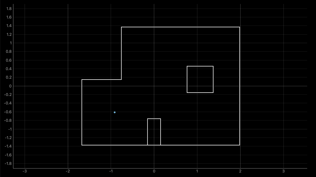
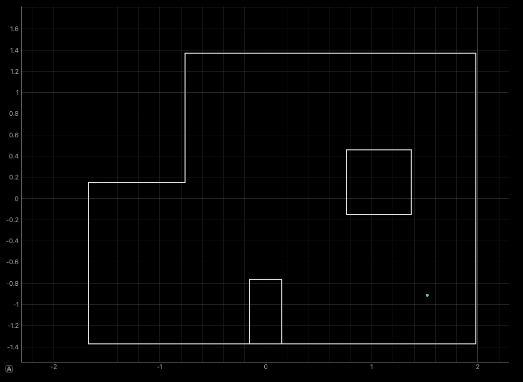
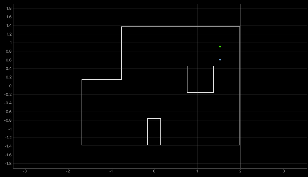
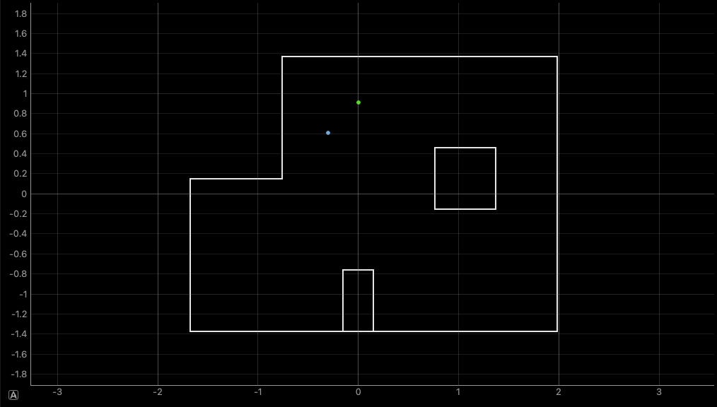
Next, to show that this all actually works, the filter is run on the robot at the marked positions in the lab:

(-3,-2)	(5,-3)
(5,3)	(0,3)

(-3,-2)	(5,-3)
(5,3)	(0,3)

From here we observe that the localization is generally pretty accurate, where it gets the position in the map right within a grid cell away. However, the filter results are still very sensitive to the starting pose of the robot, and can easily result in predictions on the other side of the map. This is not surprising, since the number of observations being used is somewhat small.

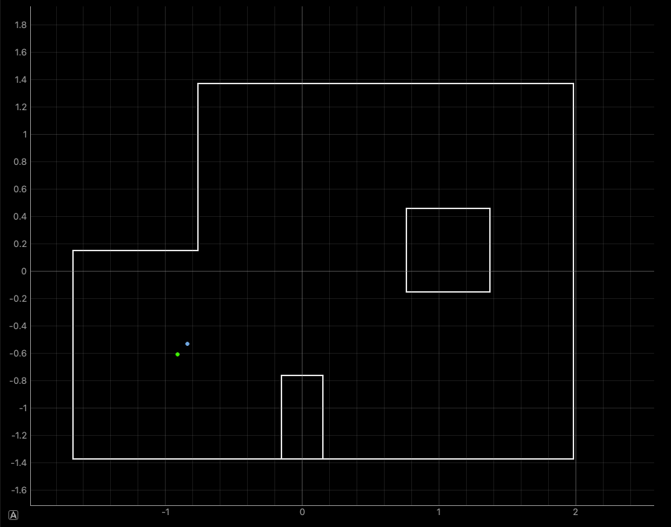
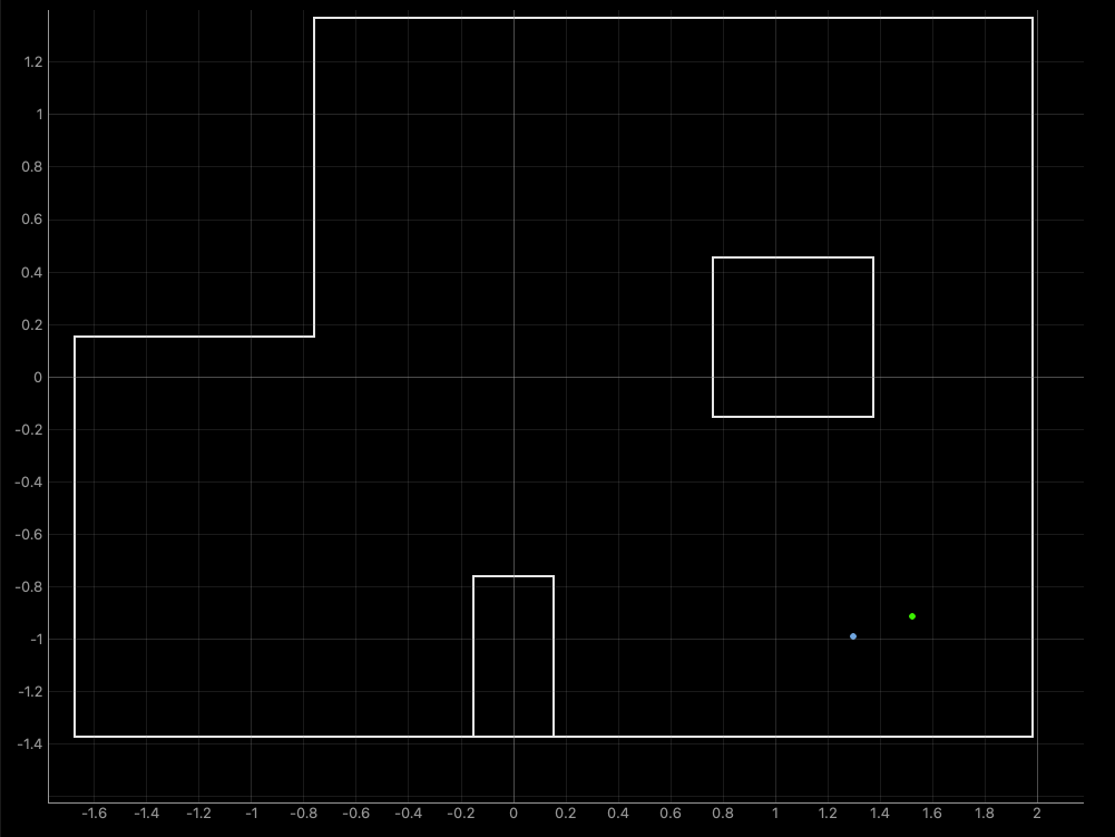
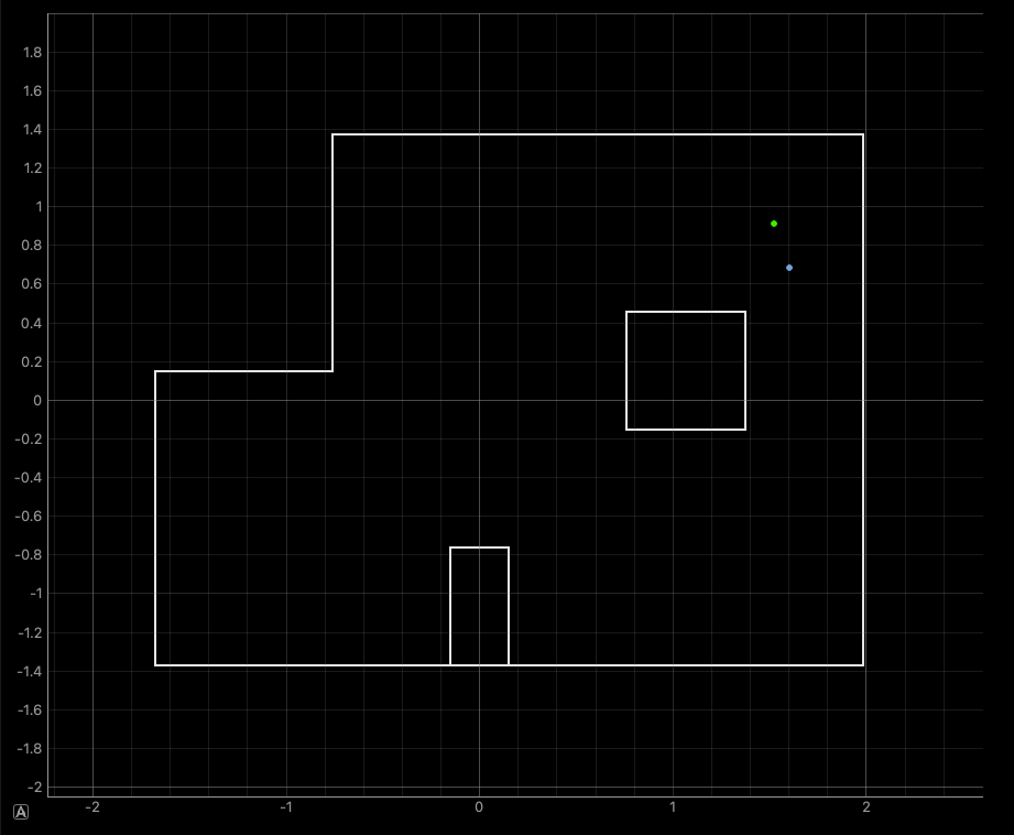
To take advantage of the improvements added through vectorizing the localization code, we double the discretization cells along $x$ and $y$, as well as increase the number of observations to 60. Increasing the number even further might still be possible, but it seems that at around 120, the probabilities from the update step become so small they round to zero.

Although the update step of the filter is generally pretty fast (under a second), the modifications to the discretization of observation counts make pre-caching the observation views per cell much slower, and can easily take up to a minute. This problem might be circumvented by simply storing the views in a pickle file and then loading them upon initializing the BaseLocalization class.

(-3,-2)	(5,-3)
(5,3)	(0,3)

(-3,-2)	(5,-3)
(5,3)	(0,3)

Based on the results above, we actually observe that the accuracy of the filter appears actually worse than before. This is somewhat misleading, since the increase of the grid discretization will in general produce more accurate results for when the marked points do not perfectly align with a grid cell like they do for this lab.

One reason for the loss in accuracy might also be due to the limited discretization along the angular dimension, which was left unchanged. Because each angle of orientation can produce very different distance measurements, it might be very tricky for a set of distance measurements to line up with the expected measurements at any one of the discretized poses.

One avenue for improvement might be to increase the angular discretization. Because this would dramatically kick up the runtime of pre-caching views as well as the prediction step up to several minutes, this would require discarding the prediction step and saving the pre-cached views to memory somehow ahead of time.

Another way to improve this might be to discard the angular pose altogether if the yaw calculated from the IMU is accurate enough. The update step would then compare distance measurements starting at a fixed yaw with distance data that would be corrected to match the correct angular orientation.